Optimizing Parameters

Introduction

In this vignette, we will illustrate how one can use a genetic algorithm to select hyperparameters for the spatial fuzzy clustering algorithm.

The proposed approach in the package (select_parameters) can be seen as a grid search method. It can be calculation intensive when the number of parameters increase. In the case of the SGFCM, three numeric parameters (alpha, beta, and m) must be selected by the user. If one decide to add a noise cluster, with also have to select delta.

If the number of clusters (k) is already selected, we can use a genetic algorithm to optimize the choice of these hyperparameters. In the case of a spatial clustering, we have two objective functions to optimize: the spatial consistency and the clusters validity.

We show here how it can be done with the package nsga2R. This method also illustrate how the two objectives are concurrent and no solution can fulfill both of them, but some solutions provide interesting compromises. For more information about the multiobjective genetic algorithm, you could check this link.

Setup

We start by loading the data and create a fitness function that will be used by the genetic algorithm.

library(geocmeans, quietly = TRUE)
library(sf, quietly = TRUE)
library(spdep, quietly = TRUE)
library(ggplot2, quietly = TRUE)
library(ggpubr, quietly = TRUE)
library(tmap, quietly = TRUE)
library(nsga2R, quietly = TRUE)
library(plotly, quietly = TRUE)

spdep::set.mcOption(FALSE)

## [1] FALSE

data(LyonIris)

AnalysisFields <-c("Lden","NO2","PM25","VegHautPrt","Pct0_14",
                   "Pct_65","Pct_Img","TxChom1564","Pct_brevet","NivVieMed")

Data <- st_drop_geometry(LyonIris[AnalysisFields])

# create the spatial weight matrix
Neighbours <- poly2nb(LyonIris,queen = TRUE)
WMat <- nb2listw(Neighbours,style="W",zero.policy = TRUE)

We try to otpimize a SGFCM with 3 parameters :

m, the fuzzyness index (limited between 1 and 2)
alpha, the weight given to the spatially lagged dataset (limited between 0 and 5)
beta, control classification crispness (between 0 and 0.99)

We want to obtain a classification with a good quality (maximizing the silhouette index) and a good spatial consistency (minimizing spatial inconsistency). We also add the explained inertia as a third objective function.

fintess_func <- function(x){
  m <- x[[1]]
  alpha <- x[[2]]
  beta <- x[[3]]
  k <- 4
  clustering <- SGFCMeans(Data,
                         WMat, 
                         k = k,
                         m = m,
                         alpha = alpha,
                         beta = beta,
                         robust = TRUE,
                         tol = 0.01,
                         standardize = TRUE,
                         verbose = FALSE,
                         maxiter = 1000,
                         seed = 123,
                         init = "kpp")
  sil <- calcSilhouetteIdx(data = clustering$Data, 
                           belongings = clustering$Belongings)
  inertia <- calcexplainedInertia(data = clustering$Data, 
                         belongmatrix = clustering$Belongings)
  space_idx <- spConsistency(clustering, nblistw = WMat, nrep = 1)
  scores <- c(-sil,  space_idx$sum_diff, -inertia)
  
  return(scores)

}

Running the genetic algorithm

This can be a long step, but this function could be easily paralellized.

results <- nsga2R(fintess_func,
                  varNo = 3,
                  objDim = 3,
                  lowerBounds = c(1,0,0),
                  upperBounds = c(2,5,0.99),
                  popSize = 200,
                  generations = 50,
                  cprob = 0.85,
                  mprob = 0.2
                  )

Analyzing the results

We combine the scores obtained in one dataframe and then we can start the analysis of the proposed solutions.

df_params <- data.frame(results$parameters)
names(df_params) <- c("m","alpha","beta")
df_scores <- data.frame(results$objectives)
names(df_scores) <- c("silhouette","space","inertia")
df_tot <- cbind(df_params, df_scores)

df_tot$silhouette <- df_tot$silhouette * -1
df_tot$inertia <- df_tot$inertia * -1
df_tot <- round(df_tot,4)


p1 <- ggplot(df_tot) + 
  geom_point(aes(x = silhouette, y = space))

p2 <- ggplot(df_tot) + 
  geom_point(aes(x = silhouette, y = inertia))

p3 <- ggplot(df_tot) + 
  geom_point(aes(x = inertia, y = space))

ggarrange(p1,p2,p3, ncol = 2, nrow = 2)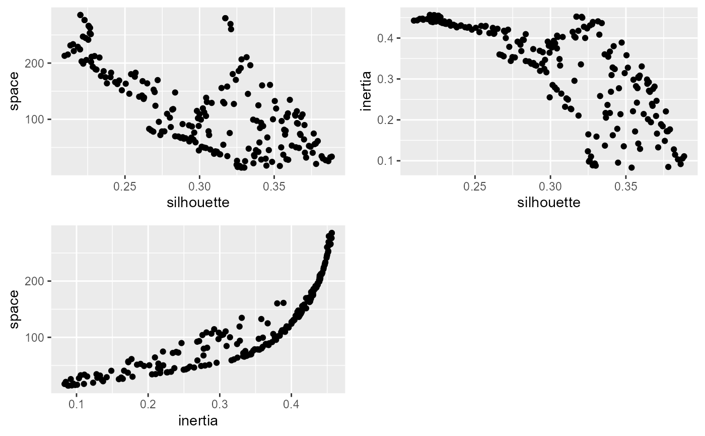

It seems that the algorithm is able to find a set of solutions that minimize simultaneously the silhouette index and the spatial inconsistency, but finding a compromise between the explained inertia and the spatial consistency is difficult.

p1 <- ggplot(df_tot) + 
  geom_point(aes(x = alpha, y = beta, color = space))

p2 <- ggplot(df_tot) + 
  geom_point(aes(x = alpha, y = m, color = space))

p3 <- ggplot(df_tot) + 
  geom_point(aes(x = alpha, y = beta, color = silhouette))

p4 <- ggplot(df_tot) + 
  geom_point(aes(x = alpha, y = m, color = silhouette))

ggarrange(p1,p2,p3,p4, ncol = 2, nrow = 2)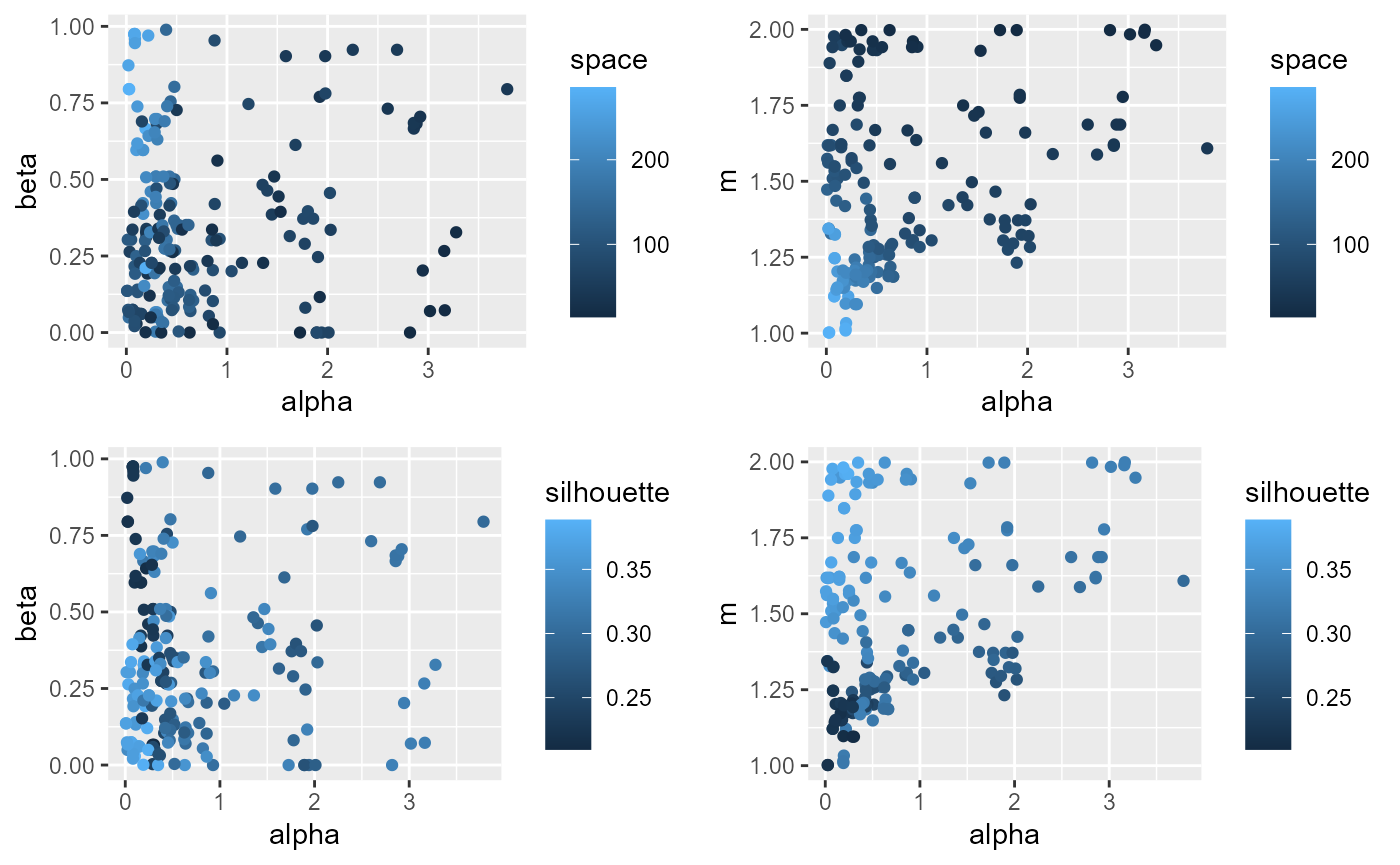

alpha is positively correlated with a lower value of spatial inconsistency, but is also negatively correlated with the silhouette index. m is positively associated with the silhouette index and the spatial consistency.

The following 3D plot clearly demonstrates the Pareto front: the set of dominant solutions. It forms a curved plane.

plot_ly(df_tot, x = ~silhouette, y = ~inertia, z = ~space) %>%
  add_markers() %>%
  add_trace(type = "mesh3d", opacity = 0.5, facecolor = "grey") %>%
  layout(scene = list(xaxis = list(title = 'silhouette'),
                     yaxis = list(title = 'explained inertia'),
                     zaxis = list(title = 'spatial inconsistency')))

To select a solution, we will limit our choices to the results with a silhouette index above 0.34 and an explained above 0.30.

solutions <- subset(df_tot,
                      df_tot$silhouette >= 0.34 & 
                      df_tot$inertia >= 0.30)

knitr::kable(solutions, digits = 2)

	m	alpha	beta	silhouette	space	inertia
9	1.47	0.01	0.14	0.36	134.64	0.33
43	1.33	0.05	0.07	0.35	161.20	0.39
50	1.44	0.10	0.25	0.35	132.52	0.36
59	1.51	0.11	0.13	0.36	104.82	0.30
75	1.52	0.11	0.14	0.36	103.89	0.30
78	1.53	0.08	0.22	0.36	110.56	0.31
97	1.52	0.19	0.27	0.35	100.09	0.31
114	1.34	0.02	0.05	0.34	160.34	0.38
122	1.48	0.09	0.19	0.35	119.19	0.33
136	1.50	0.37	0.33	0.34	88.05	0.32
153	1.54	0.30	0.47	0.34	93.92	0.33
162	1.69	0.30	0.68	0.34	84.51	0.31

We will select the one of the obtained solutions we found here. It has the rank 153 in the final set of solutions. We also compare it with the solution we selected with a grid search approach in the vignette introduction.

version1 <- SGFCMeans(Data,WMat ,k = 4,m=1.5, alpha=0.95, beta = 0.65,
                    standardize = TRUE, robust = TRUE, 
                    verbose = FALSE, seed = 123,
                    tol=0.0001, init = "kpp")

parameters <- as.list(solutions[11,])
version2 <- SGFCMeans(Data,WMat ,k = 4,
                    m = parameters$m,
                    alpha=parameters$alpha,
                    beta = parameters$beta,
                    standardize = TRUE, robust = TRUE, 
                    verbose = FALSE, seed = 123,
                    tol=0.0001, init = "kpp")

# calculating the indexes for the clustering
idx1 <- calcqualityIndexes(data = version1$Data,
                           belongmatrix = version1$Belongings,
                           m = version1$m,
                           indices = c("Silhouette.index",
                           "XieBeni.index", "FukuyamaSugeno.index",
                           "Explained.inertia"))


idx2 <- calcqualityIndexes(data = version2$Data,
                           belongmatrix = version2$Belongings,
                           m = version2$m,
                           indices = c("Silhouette.index",
                           "XieBeni.index", "FukuyamaSugeno.index",
                           "Explained.inertia"))

# calculating the spatial indexes
space1 <- spatialDiag(version1,nrep = 150)
space2 <- spatialDiag(version2,nrep = 150)

idx1$spatial.Consistency <- space1$SpConsist
idx2$spatial.Consistency <- space2$SpConsist

scores <- round(cbind(do.call(c,idx1), do.call(c,idx2)),4)
colnames(scores) <- c("reference","optimized")
scores <- data.frame(scores)
tests <- c(1, -1, -1, 1,-1)
test1 <- ifelse((scores[,1] > scores[,2]),1,-1) * tests * -1
scores$better <- ifelse(test1 == -1, FALSE, TRUE)

knitr::kable(scores)

	reference	optimized	better
Silhouette.index	0.2980	0.3403	TRUE
XieBeni.index	2.0611	1.8835	TRUE
FukuyamaSugeno.index	1976.3404	1646.7294	TRUE
Explained.inertia	0.3292	0.3281	FALSE
spatial.Consistency	0.1502	0.2241	FALSE

The optimized version gives a slightly lower spatial consistency, but also a significantly higher silhouette index.

Jeremy Gelb

14/12/2022

Introduction

Setup

Running the genetic algorithm

Analyzing the results

References