Spatial Fuzzy CMean with R

Introduction

This document is a short introduction to the package geocmeans. It implements fuzzy classification methods bringing spatial information and neighbouring in its calculation.

Note that more vignettes can be found on the website of the package:

In their article, Cai, Chen, and Zhang (2007) described the method, originally applied in the analysis of brain imagery. The generalized version of the spatial fuzzy c-means is presented by Zhao, Jiao, and Liu (2013).

Gelb and Apparicio (2021) applied the method to socio-residential and environmental data comparing the results with other unsupervised classification algorithms (in French).

There are actually numerous packages and functions to perform unsupervised classification in R (hclust, kmeans, cmeans, factoextra, etc.). However, these methods are not always well-suited to analyze spatial data. Indeed, they do not account for spatial information such as proximity or contiguity between observations. This may lead to solutions for which close observations end up in different groups event though they are very similar.

To our knowledge, the package ClustGeo is the only package proposing an unsupervised classification method which directly consider spatial proximity between observations. The proposed approach is appealing because the user can select a parameter (alpha) that controls the weight of the spatial distance matrix (calculated between observations with their locations) versus the semantic distance matrix (calculated between observations with their variables).

However, this method belongs to the category of “hard-clustering” algorithms. Each observation ends up in one cluster/group. The main draw-back here is the difficulty to identify observations that are undecided, at the frontier of two clusters/groups. The soft or fuzzy clustering algorithms provide more information because they calculate the “probability” of each observation to belong to each group.

The algorithms SFCM (spatial fuzzy c-means) and SGFCM (spatial generalized fuzzy c-means) propose to combine the best of both worlds.

The package geocmeans is an implementation in R of these methods. It comes with a set of functions to facilitate the analysis of the final membership matrices:

calculating many quality indices (coming mainly from the package fclust)
mapping the results
giving summary statistics for each cluster/group
a shiny app to investigate dynamically the results.

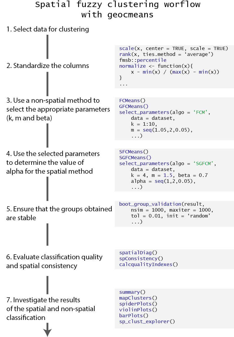
The general workflow for applying a spatial fuzzy clustering algorithm with geocmeans is described with the following figure.

Image Title

Loading the packages and the data

geocmeans comes with a toy dataset LyonIris, combining many demographic and environmental variables aggregated at the scale of the Iris (aggregated units for statistical information) in Lyon (France).

Note that the dataset used for a fuzzy classification can only contain continuous variables. For dataset with categorical variables, one could start with a PCA (Principal Component Analysis), MCA (multiple Correspondence Analysis) or a MDFA (Mixed Data Factor Analysis) and uses the obtained factors as inputs for the clustering.

Before starting the analysis, the data must be standardized because most of the calculus is based on Euclidean distance (we plan to also include Manhattan distance in a future release).

#charging packages and data
library(geocmeans)
library(ggplot2)
library(ggpubr)
library(dplyr)
library(viridis)
library(spdep)
library(tmap)

spdep::set.mcOption(FALSE)

## [1] FALSE

spdep::set.coresOption(1L)

## NULL

data(LyonIris)

# selecting the columns for the analysis
AnalysisFields <-c("Lden","NO2","PM25","VegHautPrt","Pct0_14",
                   "Pct_65","Pct_Img","TxChom1564","Pct_brevet","NivVieMed")

# rescaling the columns
Data <- sf::st_drop_geometry(LyonIris[AnalysisFields])
for (Col in names(Data)){
  Data[[Col]] <- scale(Data[[Col]])
}

Classical Kmeans

To explore the dataset and choose the right number of cluster/groups (k) we propose to start with a classical kmeans.

# finding the best k by using the r2 of the classification
# trying for k from 2 to 10
R2s <- sapply(2:10,function(k){
  Clust <- kmeans(Data,centers=k,iter.max = 150)
  R2 <- Clust$betweenss / Clust$totss
  return(R2)
})

Df <- data.frame(K=2:10,
                 R2 = R2s)

ggplot(Df)+
  geom_line(aes(x=K,y=R2s))+
  geom_point(aes(x=K,y=R2s),color="red")+
  xlab("Number of groups")+
  ylab("R2 of classification")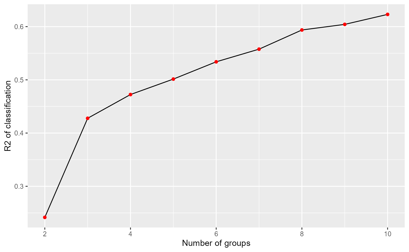

Impact of the number of groups on the explained variance

By plotting the R-squared of the kmeans classification for each k between 2 and 10, we can see a first elbow at k=3. But this small number of groups leads to a classification explaining only 43% of the original data variance. We decide to keep k=4 to have one more group in the analysis.

Let us map the obtained groups.

KMeanClust <-  kmeans(Data,centers=4,iter.max = 150)
LyonIris$Cluster <-paste("cluster",KMeanClust$cluster,sep="_")

# mapping the groups
tm_shape(LyonIris) + 
  tm_fill("Cluster", palette = c("cluster_1"="palegreen3",
                                 "cluster_2"="firebrick",
                                 "cluster_3"="lightyellow2",
                                 "cluster_4"="steelblue")) +
  tm_borders("black") +
  tm_layout(legend.outside = TRUE, frame = FALSE)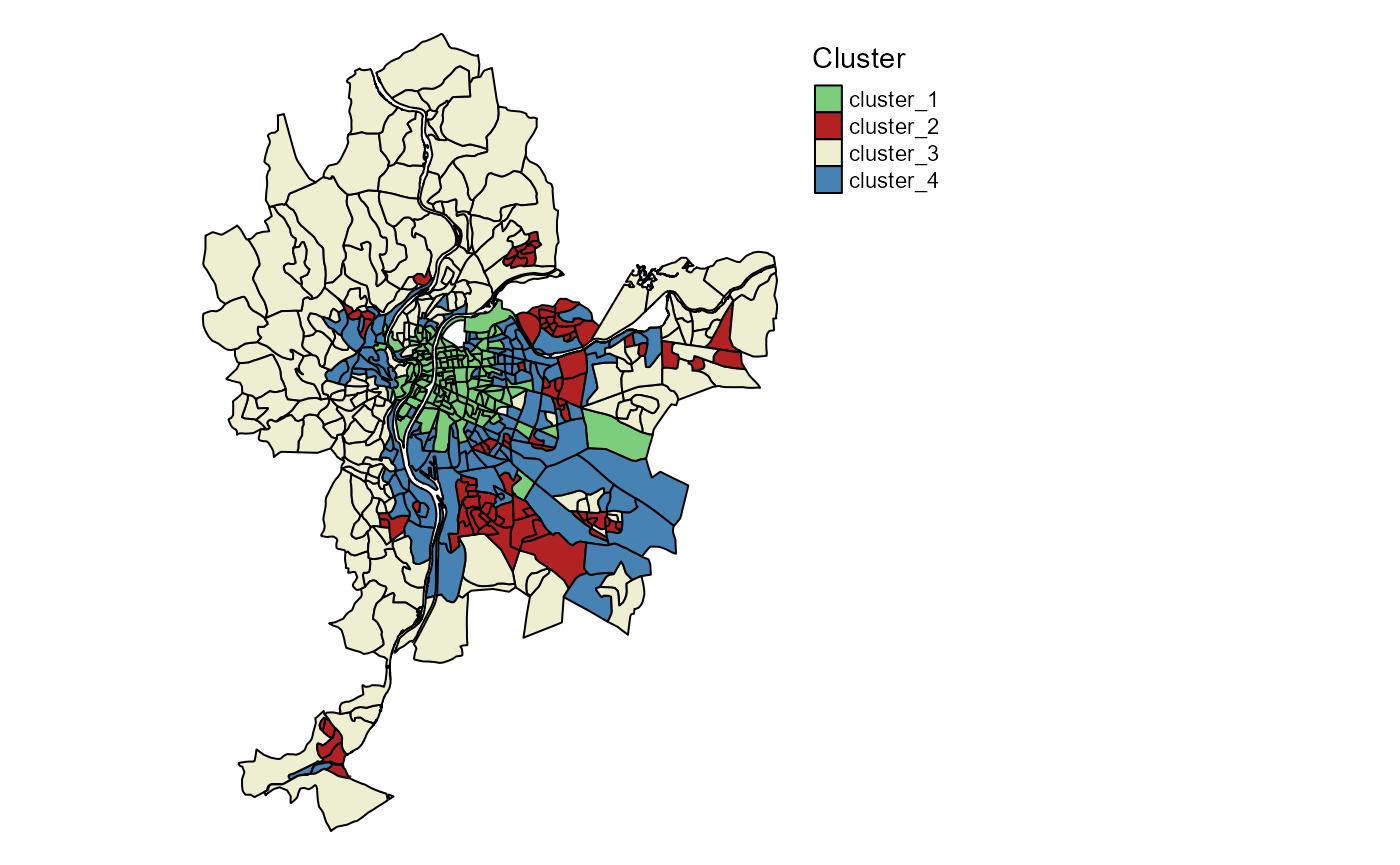

Clusters identified by classical k-means

We can clearly distinguish 4 strong spatial structures, but with some mixing between the clusters.

We could now compare this solution with a classical c-means algorithm.

Classical c-means and generalized c-means

The classical c-means is a simple method to perform fuzzy unsupervised classification. The package geocmeans proposes the function CMeans. We set the fuzziness degree (m) to 1.5.

We do not present the algorithm here, but only the two main formulas.

The first one is used to update the values of the membership matrix at each iteration \(u_ik\)

\[u_{ik} = \frac{(||x_{k} - v{_i}||^{2}) ^{(-1/(m-1))}}{\sum_{j=1}^c(||x_{k} - v{_j}||^2 )^{(-1/(m-1))}}\] And the second one to update the centers of the clusters

\[v_{i} = \frac{\sum_{k=1}^N u_{ik}^m(x_{k})}{\sum_{k=1}^N u_{ik}^m}\]

With :

\(x_k\) the values of the observation \(k\)
\(v_i\) the values of the center of the cluster \(i\)
\(c\) the number of clusters
\(m\) the fuzziness index

Cmean <- CMeans(Data,4,1.5,500,standardize = FALSE, seed = 456, tol = 0.00001, verbose = FALSE)

We can now use the function calcqualityIndexes which combines many indices from the package fclust to analyze the quality of the classification. We will use these values later for the purpose of comparisons among the different algorithms.

calcqualityIndexes(Data, Cmean$Belongings, m = 1.5)

## $Silhouette.index
## [1] 0.362851
## 
## $Partition.entropy
## [1] 0.7320161
## 
## $Partition.coeff
## [1] 0.6070524
## 
## $XieBeni.index
## [1] 1.352347
## 
## $FukuyamaSugeno.index
## [1] 1860.772
## 
## $Explained.inertia
## [1] 0.3018179

Note, geocmeans also proposes a so-called generalized version of the c-means algorithm. It is known to accelerate convergence and yield less fuzzy results by adjusting the membership matrix at each iteration. It requires an extra beta parameter controlling the strength of the modification. The modification only affects the formula updating the membership matrix.

\[u_{ik} = \frac{(||x_{k} - v{_i}||^{2} - \beta_k) ^{(-1/(m-1))}}{\sum_{j=1}^c(||x_{k} - v{_j}||^2 - \beta_k)^{(-1/(m-1))}}\]

with \(\beta_k = min(||x_{k} - v||^2)\) and \(0 \leq \beta \leq 1\).

To select an appropriate value for this parameter, we will try all the possible values between 0 and 1 with a step of 0.05.

beta_values <- selectParameters("GFCM",data = Data, k = 4, m = 1.5,
                                 beta = seq(0,1,0.05), spconsist = FALSE,
                                 tol = 0.00001, seed = 456)

knitr::kable(beta_values[c("beta","Silhouette.index","XieBeni.index","Explained.inertia")],
             col.names = c("beta", "silhouette index",
                           "Xie and Beni index", "explained inertia"),digits = 3)

beta	silhouette index	Xie and Beni index	explained inertia
0.00	0.363	1.352	0.302
0.05	0.365	1.268	0.310
0.10	0.366	1.193	0.319
0.15	0.365	1.128	0.327
0.20	0.361	1.071	0.336
0.25	0.360	1.020	0.345
0.30	0.363	0.984	0.354
0.35	0.361	0.963	0.363
0.40	0.370	0.943	0.372
0.45	0.369	0.924	0.381
0.50	0.366	0.907	0.390
0.55	0.365	0.891	0.399
0.60	0.360	0.876	0.409
0.65	0.358	0.863	0.418
0.70	0.358	0.852	0.428
0.75	0.353	0.843	0.437
0.80	0.347	0.838	0.447
0.85	0.340	0.837	0.456
0.90	0.332	0.844	0.464
0.95	0.323	0.861	0.471
1.00	0.317	0.919	0.475

Considering the table above, we select beta = 0.7, it maintains a good silhouette index, and increases Xie and Beni index and explained inertia. Let us compare the results of GFCM and FCM.

GCmean <- GCMeans(Data,k = 4,m = 1.5, beta = 0.7,500,standardize = FALSE, seed=456,
                  tol = 0.00001, verbose = FALSE)
r1 <- calcqualityIndexes(Data,GCmean$Belongings,m=1.5)
r2 <- calcqualityIndexes(Data,Cmean$Belongings,m=1.5)
df <- cbind(unlist(r1), unlist(r2))

knitr::kable(df,
             digits = 3,col.names = c("GFCM", "FCM"))

	GFCM	FCM
Silhouette.index	0.358	0.363
Partition.entropy	0.323	0.732
Partition.coeff	0.833	0.607
XieBeni.index	0.852	1.352
FukuyamaSugeno.index	585.977	1860.772
Explained.inertia	0.428	0.302

The results indicate that the GFCM provides a solution that is less fuzzy (higher explained inertia and lower partition entropy) but keeps a good silhouette index and an even better Xie and Beni index.

We can now map the two membership matrices and the most likely group for each observation. To do so, we use the function mapClusters from geocmeans. We propose here to define a threshold of 0.45. If an observation only has values below this probability in a membership matrix, it will be labeled as “undecided” (represented with transparency on the map).

We can compare the maps of the classical c-means and the generalized version.

cmeansMaps<- mapClusters(LyonIris,Cmean$Belongings,undecided = 0.45)
GcmeansMaps<- mapClusters(LyonIris,GCmean$Belongings,undecided = 0.45)

tmap_arrange(cmeansMaps$ProbaMaps[[1]],GcmeansMaps$ProbaMaps[[1]], nrow = 1, ncol = 2)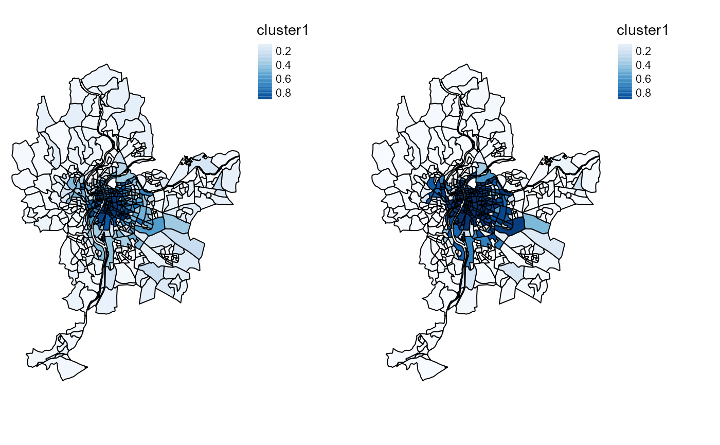

Probability of belonging to cluster 1

tmap_arrange(cmeansMaps$ProbaMaps[[2]],GcmeansMaps$ProbaMaps[[2]], 
          nrow = 1, ncol = 2)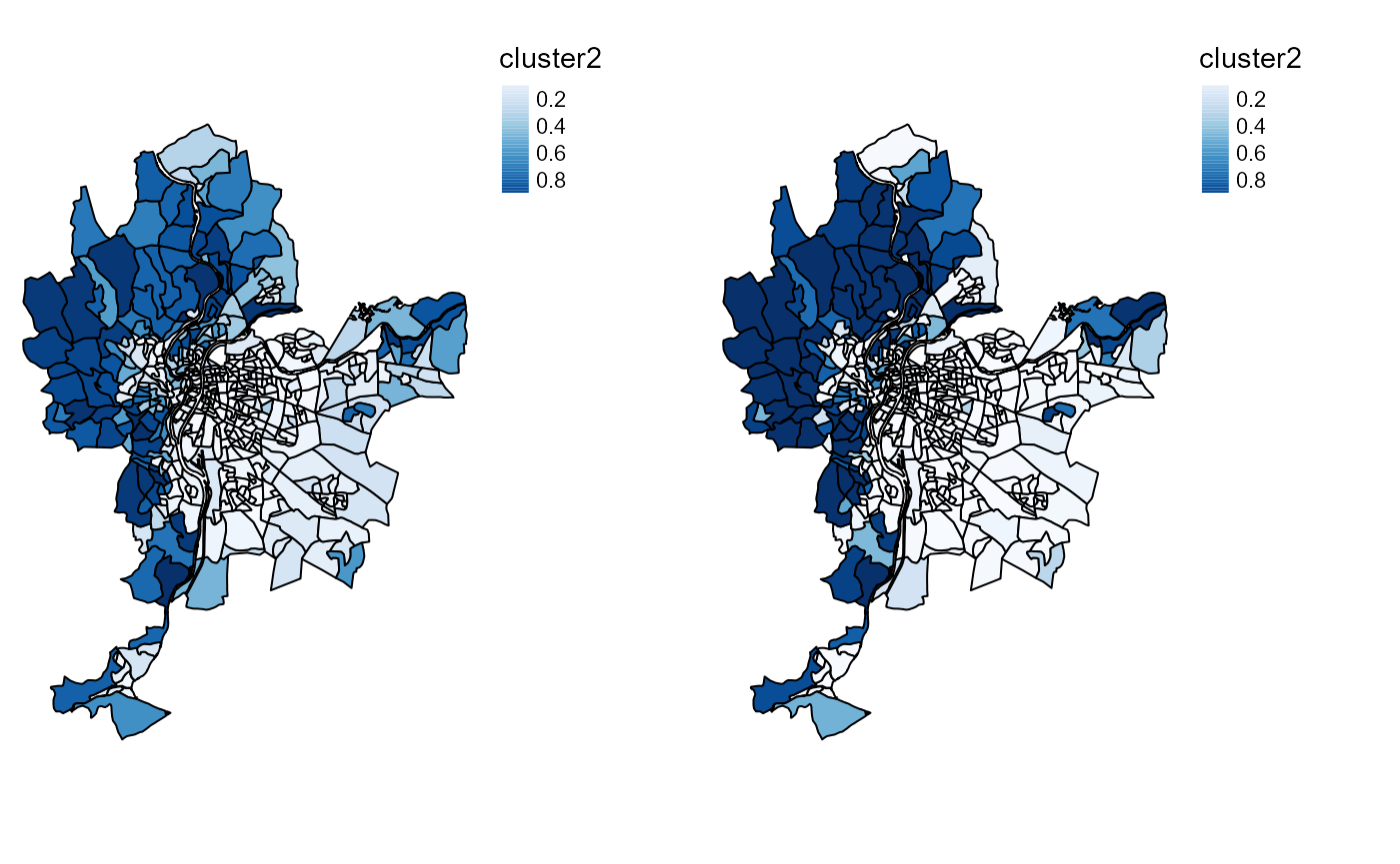

Probability of belonging to cluster 2

tmap_arrange(cmeansMaps$ProbaMaps[[3]],GcmeansMaps$ProbaMaps[[3]], 
          nrow = 1, ncol = 2)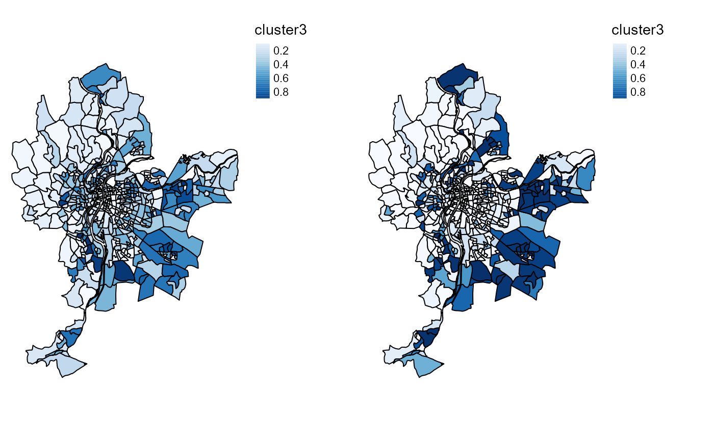

Probability of belonging to cluster 3

tmap_arrange(cmeansMaps$ProbaMaps[[4]],GcmeansMaps$ProbaMaps[[4]], 
          nrow = 1, ncol = 2)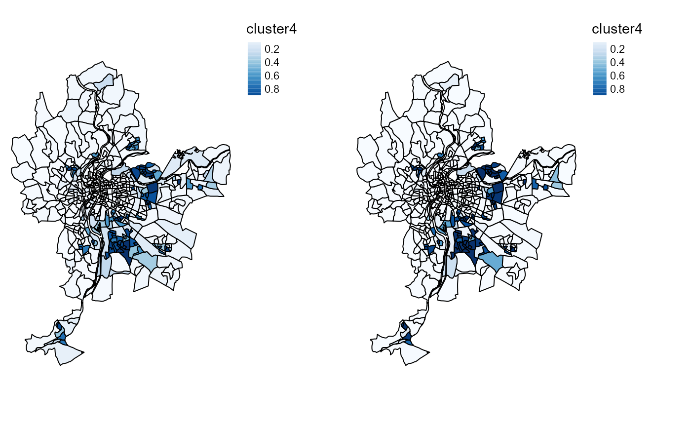

Probability of belonging to cluster 4

tmap_arrange(cmeansMaps$ClusterPlot,GcmeansMaps$ClusterPlot,
          nrow = 1, ncol = 2)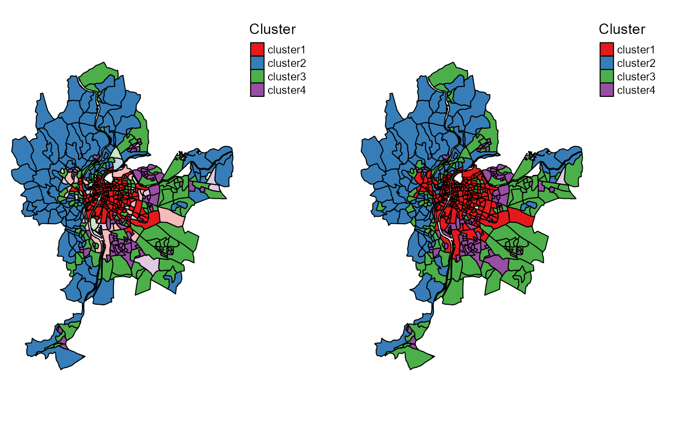

Most likely clusters and undecided units

As expected, the results are very similar, but the generalized version provides a more clear-cut classification.

Spatial c-means and generalized c-means

Selecting alpha for SFCM

Now we can use the SFCM function to perform a spatial c-means. The first step is to define a spatial weight matrix indicating which observations are neighbours and the strength of their relationship. We propose here to use a basic queen neighbour matrix (built with spdep). The matrix must be row-standardized to ensure that the interpretation of all the parameters remains clear.

Neighbours <- poly2nb(LyonIris,queen = TRUE)
WMat <- nb2listw(Neighbours,style="W",zero.policy = TRUE)

The main challenge with the SFCM method is to select the parameter alpha. It represents the weight of the spatial dimension (lagged values) in the calculus of the membership matrix and the cluster centers.

If alpha=0, then we end up with a classical c-means algorithm.
If alpha=1, then the original and the lagged values have the same weight
If alpha=2, then the lagged values are twice more important than the original values
end so on…

The two following formulas show how the functions updating the membership matrix and the centers of the clusters are modified.

\[u_{ik} = \frac{(||x_{k} - v{_i}||^2 + \alpha||\bar{x_{k}} - v{_i}||^2)^{(-1/(m-1))}}{\sum_{j=1}^c(||x_{k} - v{_j}||^2 + \alpha||\bar{x_{k}} - v{_j}||^2)^{(-1/(m-1))}}\]

\[v_{i} = \frac{\sum_{k=1}^N u_{ik}^m(x_{k} + \alpha\bar{x_{k}})}{(1 + \alpha)\sum_{k=1}^N u_{ik}^m}\] with \(\bar{x}\) the lagged version of x and \(\alpha \geq 0\)

As the formula suggests, the SFCM can be seen as a spatially smoothed version of the classical c-means and alpha controls the degree of spatial smoothness. This smoothing can be interpreted as an attempt to reduce spatial overfitting of the classical c-means.

To select alpha, we propose to check all possible values between 0 and 2 with a step of 0.05.

DFindices_SFCM <- selectParameters(algo = "SFCM", data = Data,
                               k = 4, m = 1.5, alpha = seq(0,2,0.05),
                               nblistw = WMat, standardize = FALSE,
                               tol = 0.0001, verbose = FALSE, seed = 456)

Now we are able to check the indices to select the best alpha. The goal is to reduce spatial inconsistency as much as possible and to maintain a good classification quality.

Let us start with the spatial inconsistency. This indicator (developed for this package) calculates the sum of the squared differences between each observation and its neighbours on the membership matrix. Thus, the maximum for each observation is \(k*j\) with j the number of neighbours for the observation and k the number of groups. A maximum is reached if each observation has 100% chance belonging to a cluster that is different from all its neighbours. So, when we sum up the values obtained for all the observations, we obtain a quantity of spatial inconsistency. This quantity is divided by the quantity obtained when randomly permuting the rows of the membership matrix. This second quantity represents the spatial inconsistency that we might expect if the observations were randomly scattered in space. We can repeat the permutation step (Monte Carlo approach) and keep the mean of the ratios to have a more robust indicator (see help(spConsistency) for details).

A smaller value indicates a smaller spatial inconsistency and thus a greater spatial consistency. 0 meaning that all observations have exactly the same values in the membership matrix as their neighbours (perfect spatial consistency).

ggplot(DFindices_SFCM)+
  geom_smooth(aes(x=alpha,y=spConsistency), color = "black")+
  geom_point(aes(x=alpha,y=spConsistency), color = "red")

## `geom_smooth()` using method = 'loess' and formula = 'y ~ x'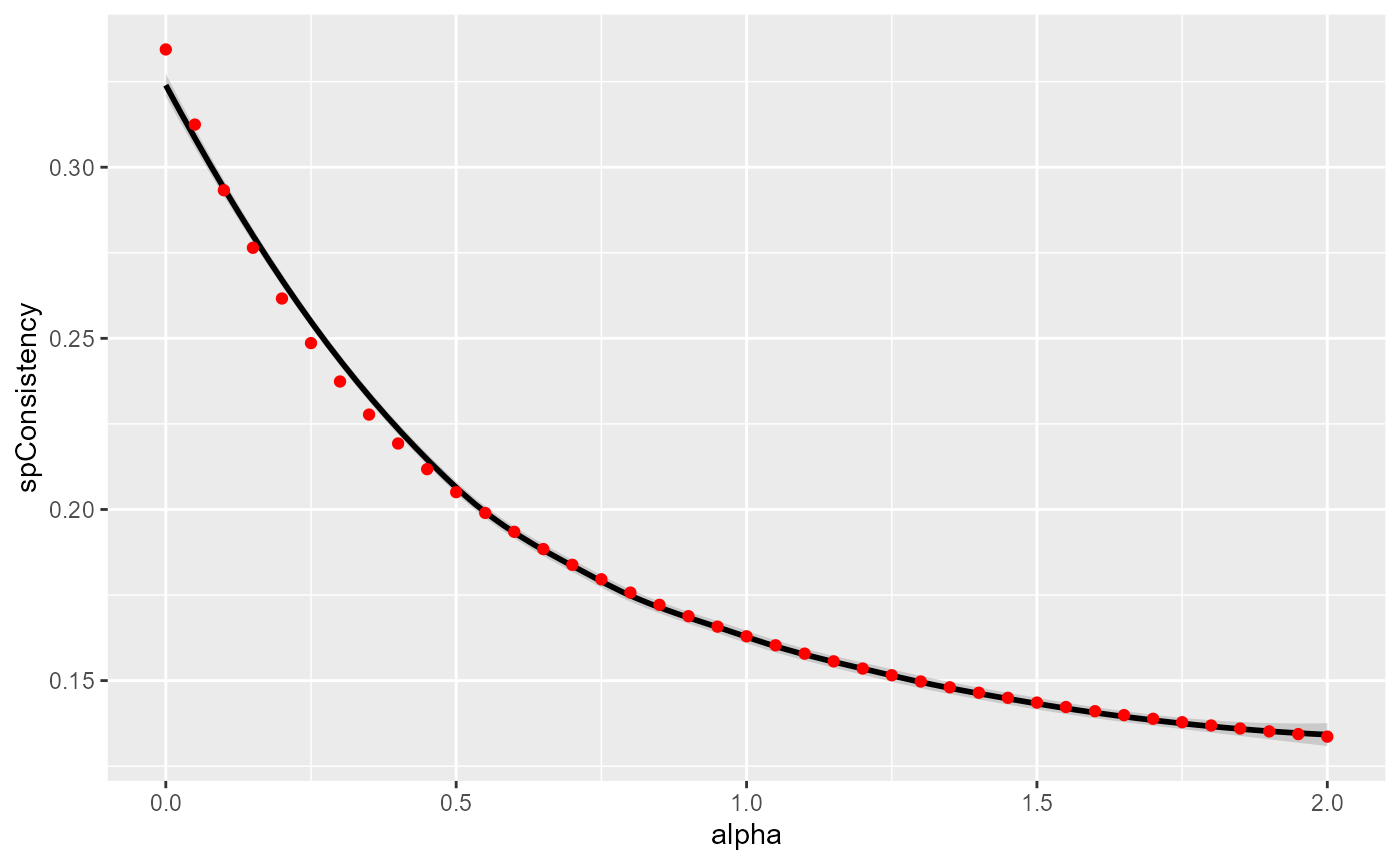

Link between alpha and spatial inconsistency

Not surprisingly, increasing alpha leads to a decrease of the spatial inconsistency. This gain follows an inverse function.

Let us now check the explained inertia

ggplot(DFindices_SFCM)+
  geom_smooth(aes(x=alpha,y=Explained.inertia), color = "black")+
  geom_point(aes(x=alpha,y=Explained.inertia), color = "red")

## `geom_smooth()` using method = 'loess' and formula = 'y ~ x'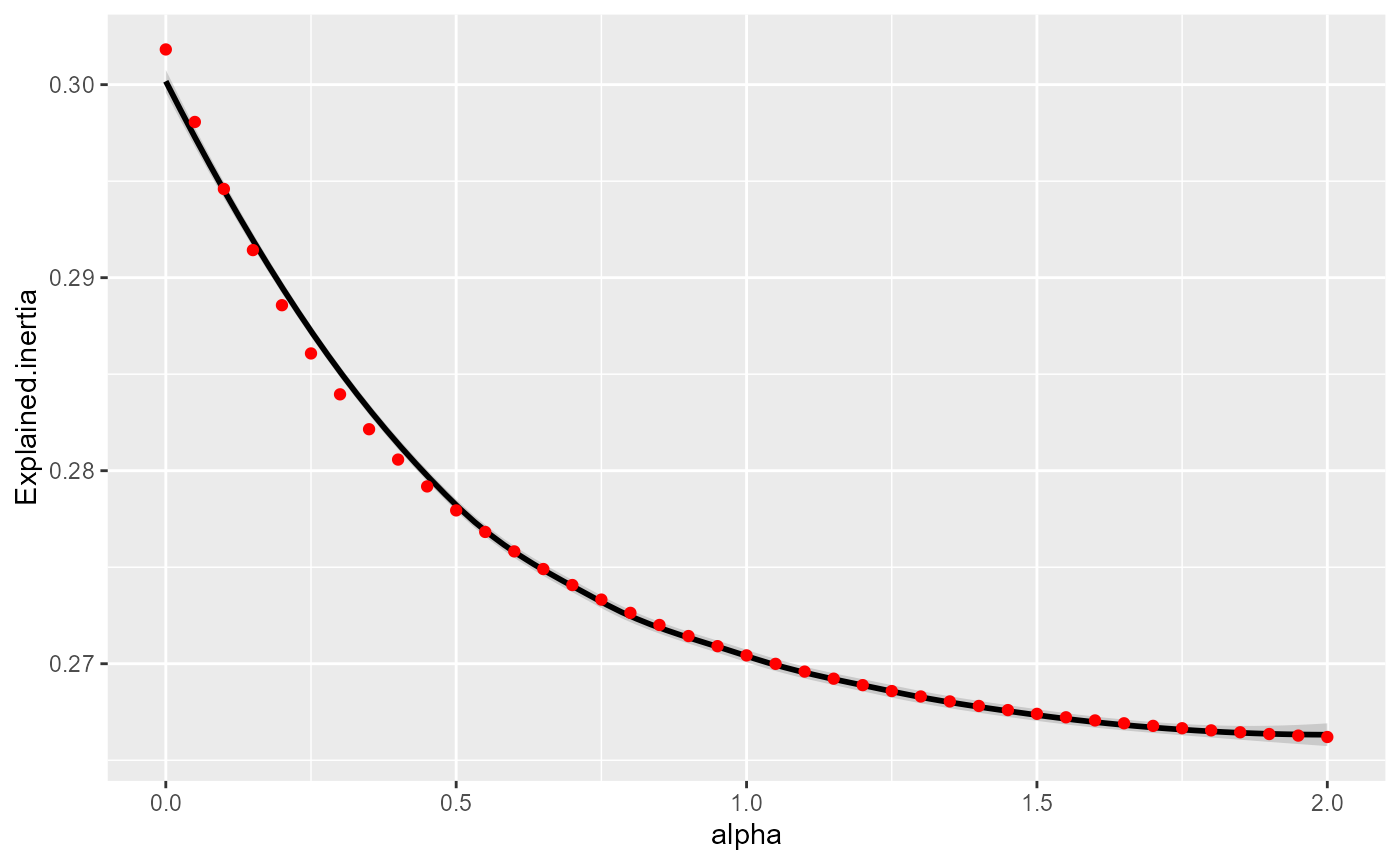

Link between alpha and explained inertia

As expected, the explained inertia decreases when alpha increases and again follows an inverse function. The classification has to find a compromise between the original values and the lagged values. However, the loss is very small here: only 3% between alpha = 0 and alpha = 2.

To finish here, we can observe the silhouette and Xie and Beni indicators.

ggplot(DFindices_SFCM)+
  geom_smooth(aes(x=alpha,y=Silhouette.index), color = "black")+
  geom_point(aes(x=alpha,y=Silhouette.index), color = "red")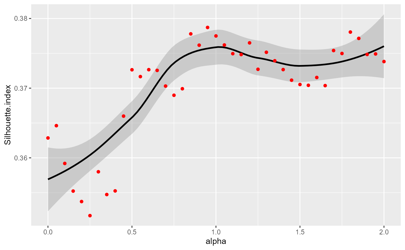

Link between alpha and silhouette index

ggplot(DFindices_SFCM)+
  geom_smooth(aes(x=alpha,y=XieBeni.index), color = "black")+
  geom_point(aes(x=alpha,y=XieBeni.index), color = "red")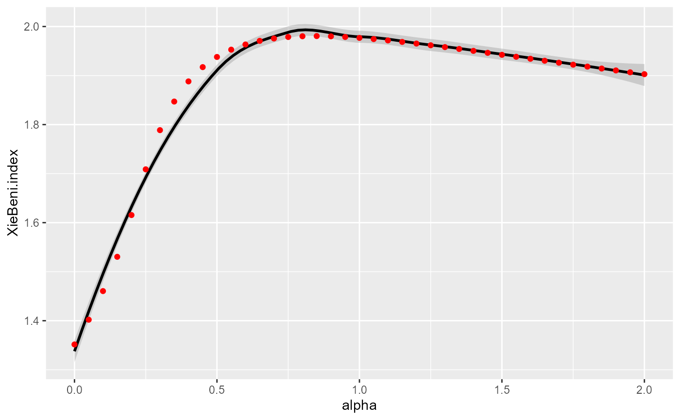

Link between alpha and Xie and Beni index

The detail of the meaning of these indicators is beyond the scope of this vignette. Let us just stress that a larger silhouette index indicates a better classification, and a smaller Xie and Beni index indicates a better classification.

After considering all the previous charts, we decide to keep alpha = 0.7 as it seems to provide a good balance between spatial consistency and classification quality in this case.

SFCM <- SFCMeans(Data, WMat, k = 4, m = 1.5, alpha = 0.7,
                 tol = 0.0001, standardize = FALSE,
                 verbose = FALSE, seed = 456)

Selecting alpha and beta for SGFCM

It is also possible to use the so-called generalized version of the spatial c-means. In that case, we must define both alpha and beta.

The next formula shows how the membership matrix is updated at each iteration. Note that the centres of the clusters are updated with the same formula as SFCM.

\[u_{ik} = \frac{(||x_{k} - v{_i}||^2 -\beta_k + \alpha||\bar{x_{k}} - v{_i}||^2)^{(-1/(m-1))}}{\sum_{j=1}^c(||x_{k} - v{_j}||^2 -\beta_k + \alpha||\bar{x_{k}} - v{_j}||^2)^{(-1/(m-1))}}\]

Because we select a high resolution for our grid search of alpha and beta, we will use a multiprocessing approach.

future::plan(future::multisession(workers=2))
DFindices_SFGCM <- selectParameters.mc(algo = "SGFCM", data = Data,
                               k = 4, m = 1.5, alpha = seq(0,2,0.05),
                               beta = seq(0,0.85,0.05),
                               nblistw = WMat, standardize = FALSE, chunk_size = 50,
                               tol = 0.0001, verbose = FALSE, seed = 456)

ggplot(DFindices_SFGCM) + 
  geom_raster(aes(x = alpha, y = beta, fill = Silhouette.index),  size = 5) + 
  scale_fill_viridis() +
  coord_fixed(ratio=1)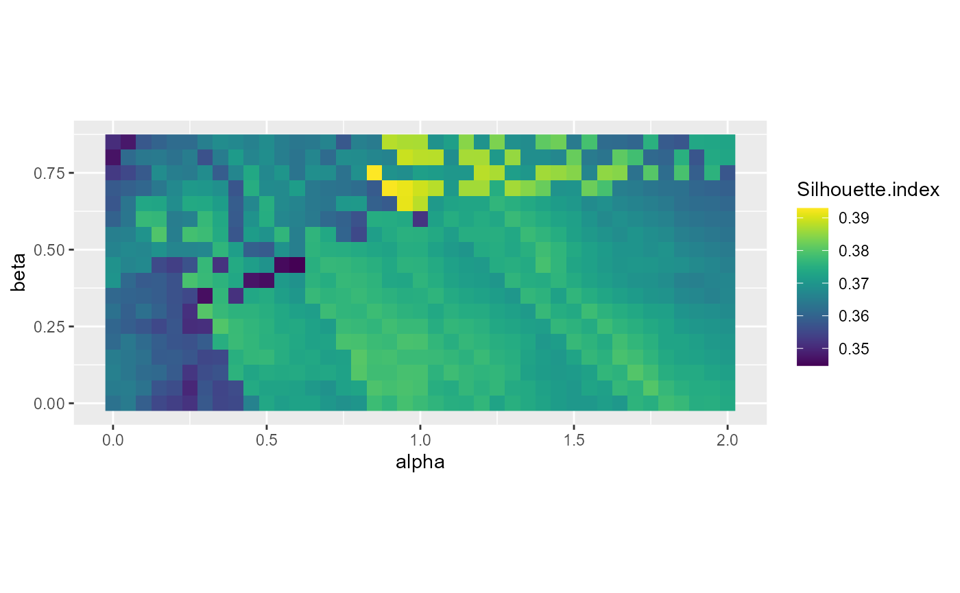

Impact of beta and alpha on silhouette index

ggplot(DFindices_SFGCM) + 
  geom_raster(aes(x = alpha, y = beta, fill = XieBeni.index),  size = 5) + 
  scale_fill_viridis() +
  coord_fixed(ratio=1)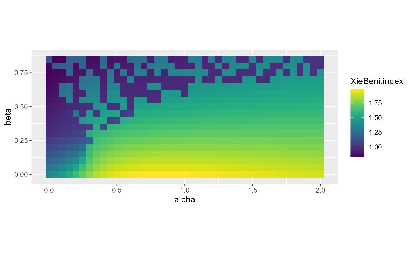

Impact of beta and alpha on Xie and Beni index

ggplot(DFindices_SFGCM) + 
  geom_raster(aes(x = alpha, y = beta, fill = spConsistency),  size = 5) + 
  scale_fill_viridis() +
  coord_fixed(ratio=1)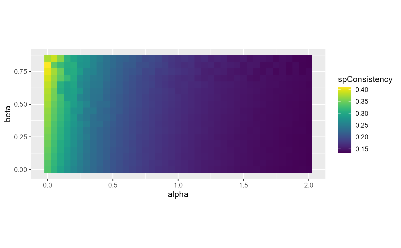

Impact of beta and alpha on spatial inconsistency

The first two plots indicate that some specific pairs of alpha and beta yield good results in the range 0.8 < alpha < 1.2 and 0.6 < beta < 0.8. The last plot shows that the selection of beta has no impact on the spatial consistency.

Considering the previous plots, we decide to retain the solution with beta = 0.65 and alpha = 0.95 which yield very good results for all the indices considered.

SGFCM <- SGFCMeans(Data,WMat,k = 4,m=1.5, alpha=0.95, beta = 0.65,
                    tol=0.0001, standardize = FALSE, verbose = FALSE, seed = 456)

Again, we compare here the generalized and the classical version of the spatial c-means algorithm.

r1 <- calcqualityIndexes(Data, SFCM$Belongings,m = 1.5)
r2 <- calcqualityIndexes(Data, SGFCM$Belongings,m = 1.5)

diagSFCM <- spatialDiag(SFCM$Belongings, nblistw = WMat,
                        undecided = 0.45,nrep = 500)
diagSGFCM <- spatialDiag(SGFCM$Belongings, nblistw = WMat,
                         undecided = 0.45,nrep = 500)

df <- cbind(
  c(unlist(r1),diagSFCM$SpConsist),
  c(unlist(r2),diagSGFCM$SpConsist)
)
row.names(df)[length(row.names(df))] <- "sp.consistency"

knitr::kable(df,digits = 3,col.names = c("SFCM","SGFCM"))

	SFCM	SGFCM
Silhouette.index	0.370	0.391
Partition.entropy	0.765	0.544
Partition.coeff	0.592	0.715
XieBeni.index	1.976	0.971
FukuyamaSugeno.index	2228.507	1585.559
Explained.inertia	0.274	0.347
sp.consistency	0.183	0.171

The solution of the SGFCM is better on the semantic and the spatial aspects.

We can compare the maps

SFCMMaps <- mapClusters(geodata = LyonIris, object = SFCM$Belongings,undecided = 0.45)
SGFCMMaps <- mapClusters(geodata = LyonIris, object = SGFCM$Belongings,undecided = 0.45)

tmap_arrange(SFCMMaps$ProbaMaps[[1]],SGFCMMaps$ProbaMaps[[1]],
             nrow = 1, ncol = 2)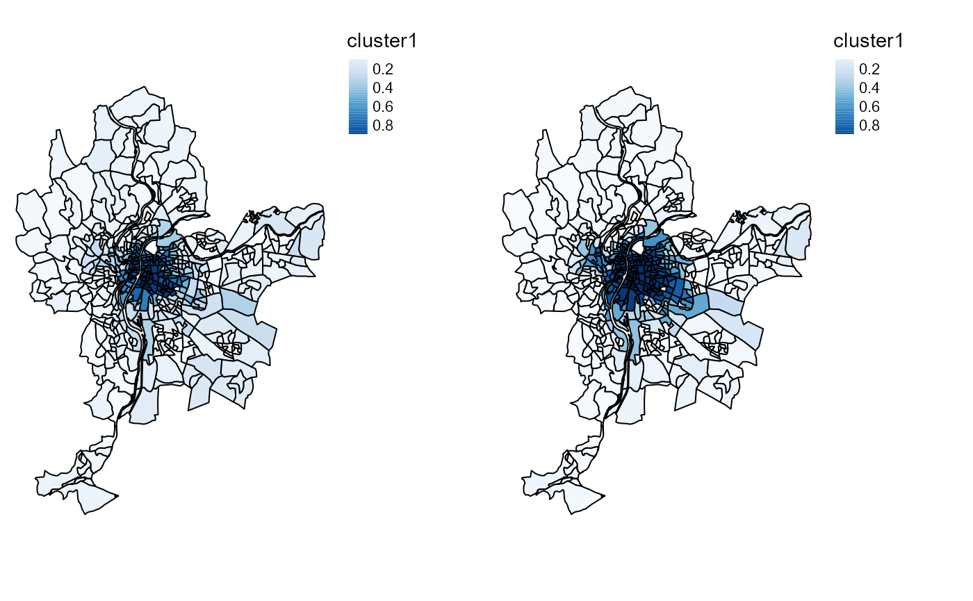

Probability of belonging to cluster 1

tmap_arrange(SFCMMaps$ProbaMaps[[2]],SGFCMMaps$ProbaMaps[[2]],
             nrow = 1, ncol = 2)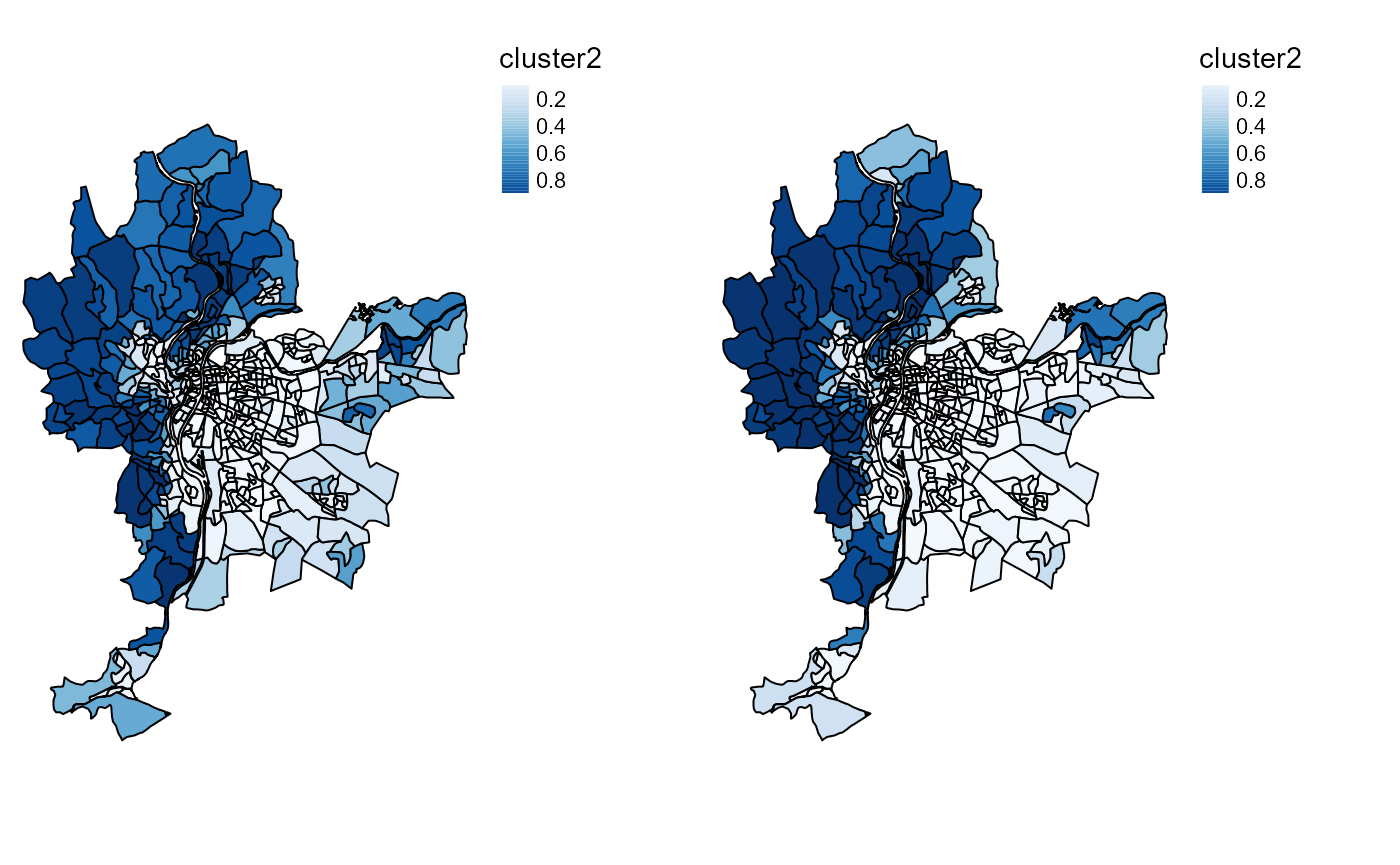

Probability of belonging to cluster 2

tmap_arrange(SFCMMaps$ProbaMaps[[3]],SGFCMMaps$ProbaMaps[[3]],
             nrow = 1, ncol = 2)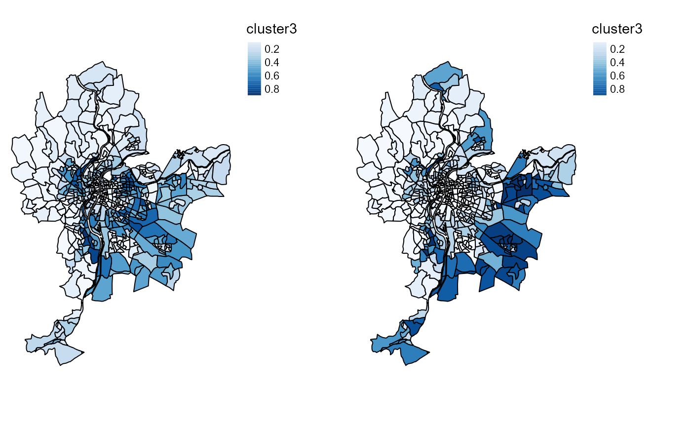

Probability of belonging to cluster 3

tmap_arrange(SFCMMaps$ProbaMaps[[4]],SGFCMMaps$ProbaMaps[[4]],
             nrow = 1, ncol = 2)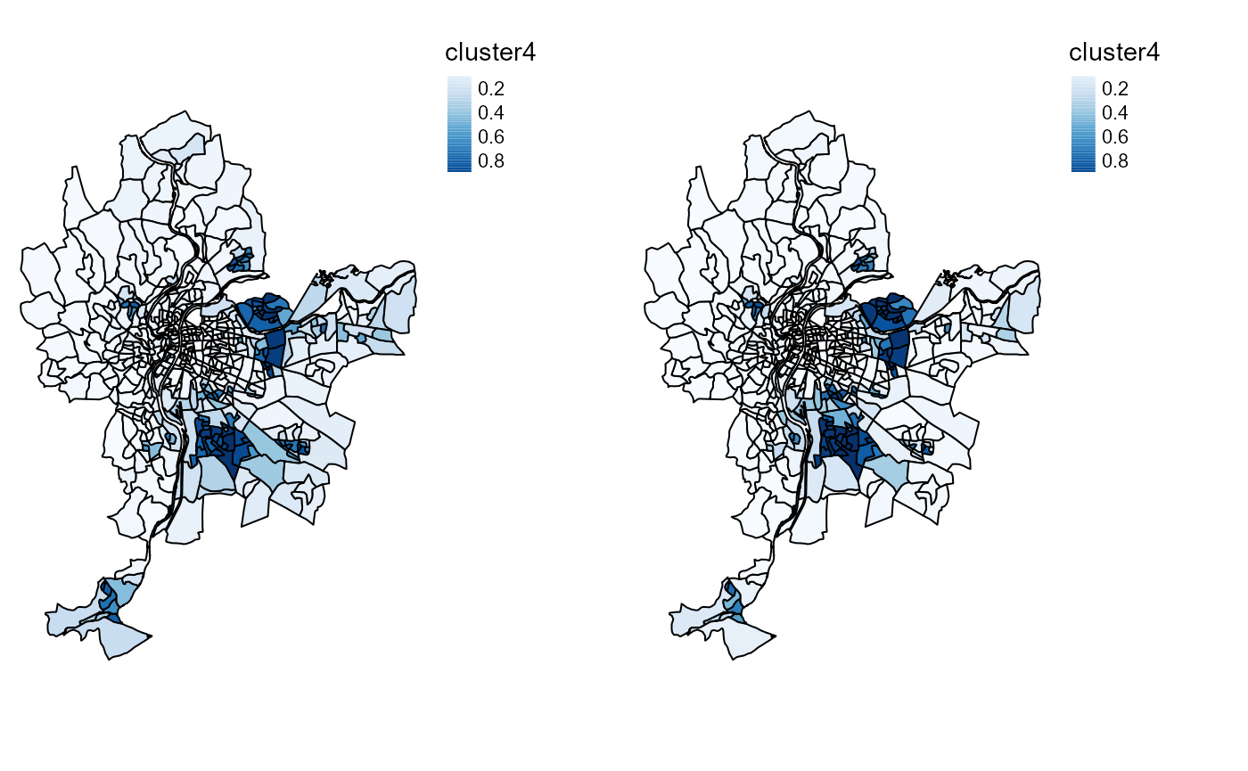

Probability of belonging to cluster 4

tmap_arrange(SFCMMaps$ClusterPlot,SGFCMMaps$ClusterPlot,
             nrow = 1, ncol = 2)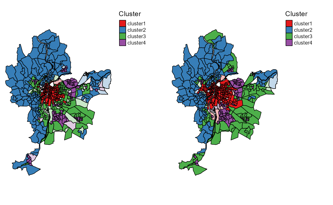

Most likely cluster and undecided units

Comparing the spatial consistency of FCM, GFCM, SFCM and SGFCM

Now, we can do a deeper spatial analysis and compare the spatial consistency of the four classifications realized (FCM, GFCM, SFCM, SGFCM).

spdiag_1 <- spatialDiag(Cmean$Belongings, nblistw = WMat, nrep=250)
spdiag_2 <- spatialDiag(GCmean$Belongings, nblistw = WMat, nrep=250)
spdiag_3 <- spatialDiag(SFCM$Belongings, nblistw = WMat, nrep=250)
spdiag_4 <- spatialDiag(SGFCM$Belongings, nblistw = WMat, nrep=250)

#looking at the moran I values for each group
moran_table <- data.frame(cbind(spdiag_1$MoranValues$MoranI,
                     spdiag_2$MoranValues$MoranI,
                     spdiag_3$MoranValues$MoranI,
                     spdiag_4$MoranValues$MoranI
                     ))
row.names(moran_table) <- paste("cluster ",1:4,sep="")
knitr::kable(moran_table, digits = 3,
             col.names = c("FCM","GFCM","SFCM","SGFCM"),
             caption = "Moran I index for the columns of the membership matrix"
             )

Moran I index for the columns of the membership matrix
	FCM	GFCM	SFCM	SGFCM
cluster 1	0.835	0.789	0.908	0.913
cluster 2	0.723	0.624	0.860	0.865
cluster 3	0.389	0.408	0.645	0.703
cluster 4	0.547	0.489	0.749	0.741

Not surprisingly, the Moran I values calculated on the membership matrices are higher for SFCM and SGFCM, indicating stronger spatial structures in the classifications.

print(c(spdiag_1$SpConsist, spdiag_2$SpConsist,spdiag_3$SpConsist,spdiag_4$SpConsist))

## [1] 0.3344399 0.3933804 0.1837933 0.1713737

Considering the values of spatial inconsistency, we could check if the value obtained for SGFCM is significantly lower than the one of SFCM. Considering the previous 250 values obtained by permutations, we can calculate a pseudo p-value:

sum(spdiag_4$SpConsist > spdiag_3$SpConsistSamples) / length(spdiag_3$SpConsistSamples)

## [1] 0

It appears that out of 250 permutations, the observed values of spatial inconsistency of SGFCM are always lower than that of SFCM. The difference is significant at the threshold 0.004 (=1/250)

We can map the undecided observations of the final solution. These entities should be analyzed more precisely. Selecting them is easy with the function undecidedUnits of the geocmeans package.

Undecided <- undecidedUnits(SGFCM$Belongings,0.45)
LyonIris$FinalCluster <- ifelse(Undecided=="Undecided",
                                "Undecided",paste("cluster",Undecided,sep="_"))

# mapping the groups
tm_shape(LyonIris) + 
  tm_fill("FinalCluster", palette = c("cluster_V1"="palegreen3",
                                 "cluster_V2"="firebrick",
                                 "cluster_V3"="lightyellow2",
                                 "cluster_V4"="steelblue",
                                 "cluster_V5"="pink",
                                 "Undecided"=rgb(0,0,0,0.4))) + 
  tm_borders("black") + 
  tm_layout(frame = FALSE, legend.outside = TRUE)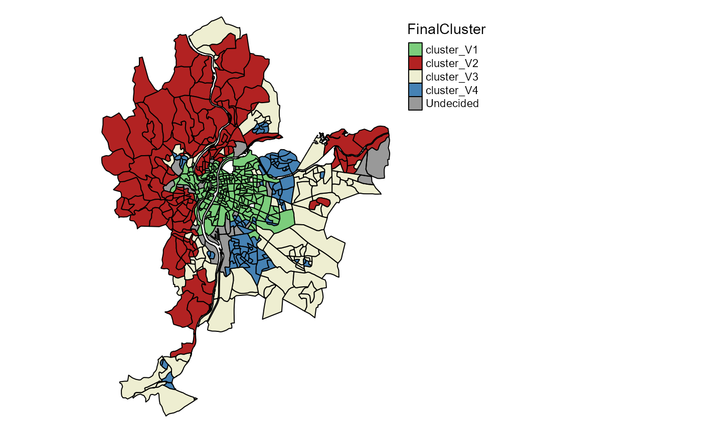

It is also possible to visualize the uncertainty by using jittered points. The idea is to draw random points in polygons and attribute them to a group proportionally to the membership values of the polygon the fall in.

colors <- c("palegreen3","firebrick","lightyellow2","steelblue","pink")
uncertaintyMap(LyonIris, SGFCM$Belongings, color = colors)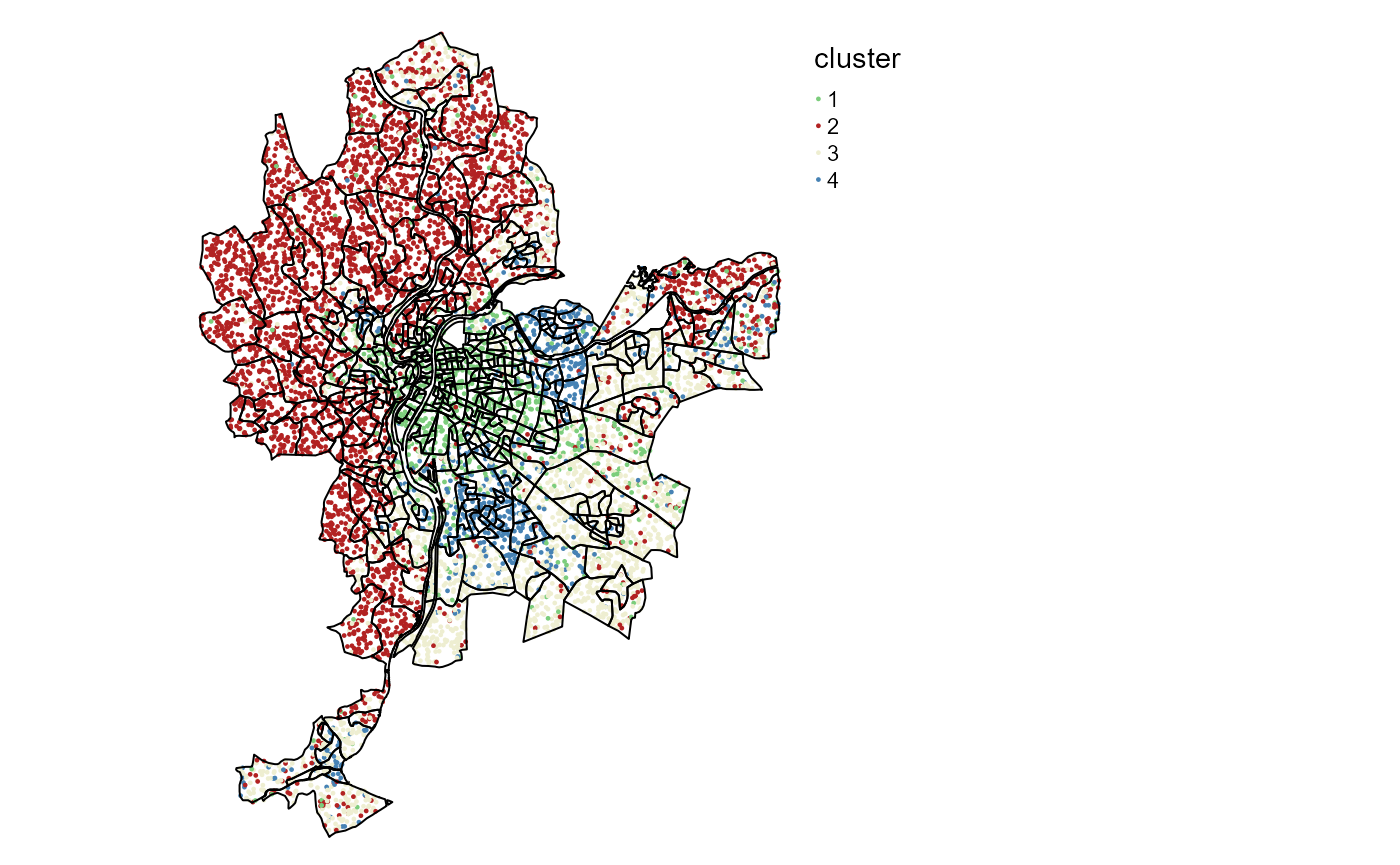

To quantify and map uncertainty, one could Calculate the Shanon entropy index and use it as a measure of uncertainty with the function calcUncertaintyIndex. A value of 1 indicates that an observation has equal membership values among groups and a value of 0 indicates that an observation belongs to only one group.

LyonIris$entropyidx  <- calcUncertaintyIndex(SGFCM$Belongings)

# mapping the uncertainty
tm_shape(LyonIris) + 
  tm_fill("entropyidx", palette = "Greys", style = "cont") + 
  tm_borders("black") + 
  tm_layout(frame = FALSE, legend.outside = TRUE)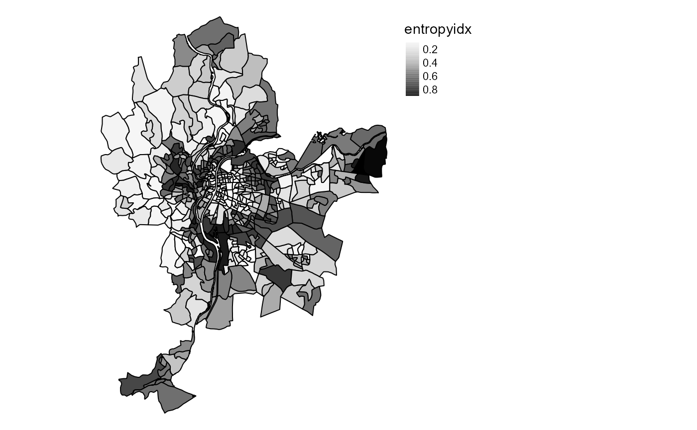

Interpreting the results of the final classification

One can obtain a lot of descriptive information about the final groups with four functions of geocmeans :

summarizeClusters: calculate summary statistics for each group for a given dataset by using the membership matrix as weights (sticking with the fuzzy spirit). One can also use the generic function summary
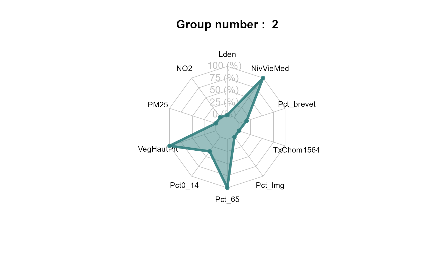
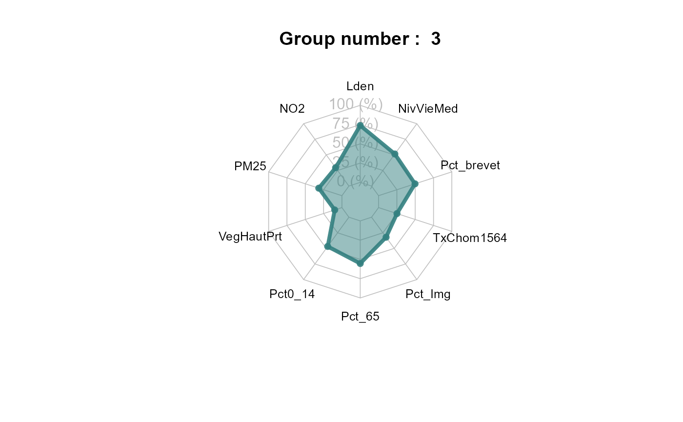
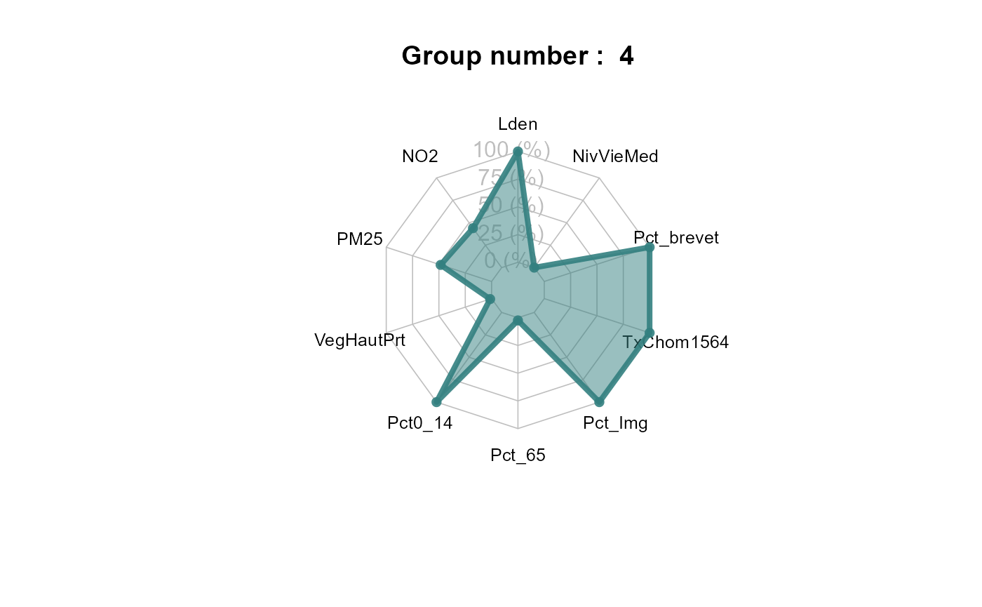
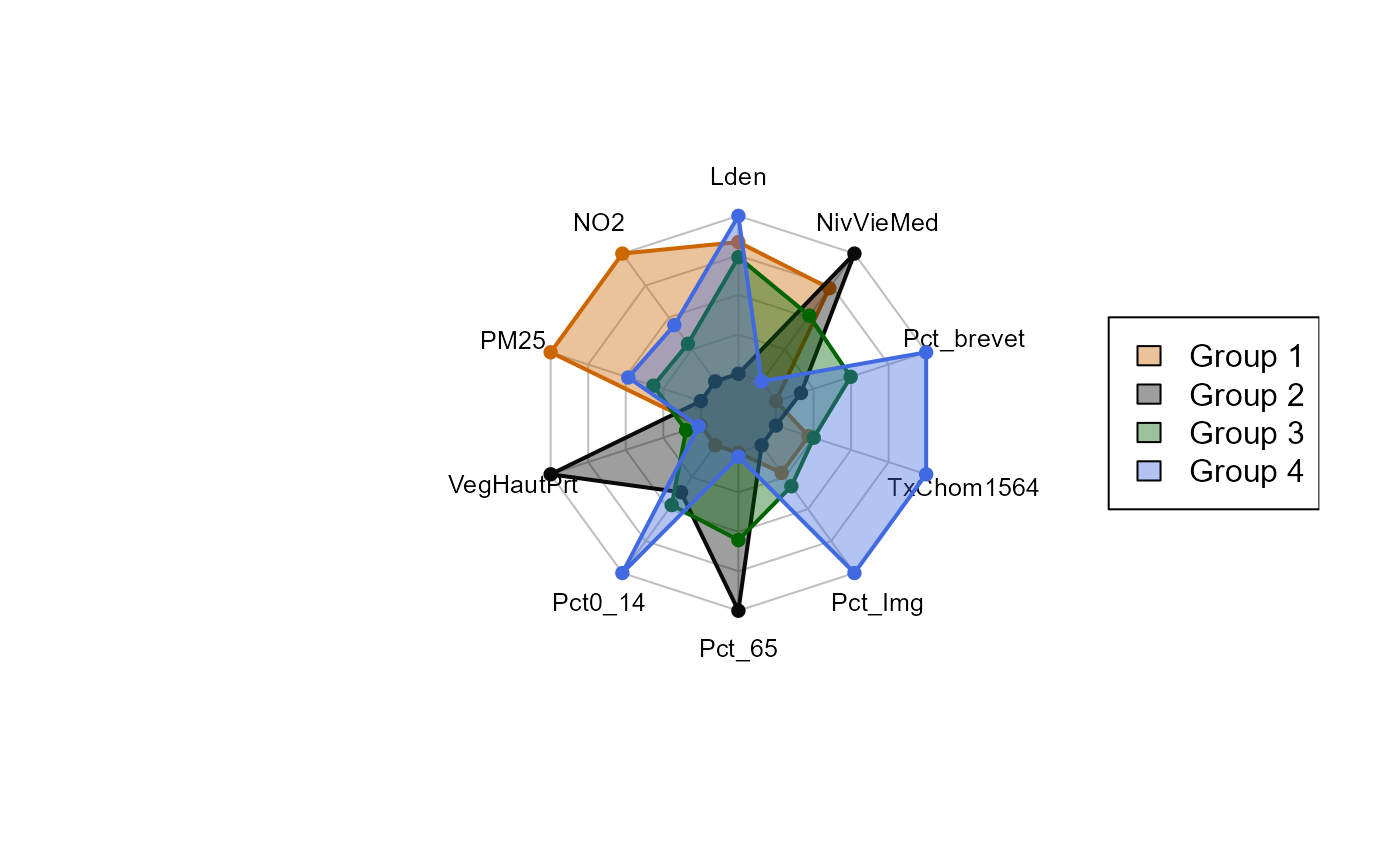
spiderPlots: display a spider plot allowing to compare quickly the differences between groups.
violinPlots: display a violin plot for each variable in a given dataset. Observations must be grouped before.
sp_clust_explorer: launch a shiny app to investigate the results dynamically.

Data <- sf::st_drop_geometry(LyonIris[AnalysisFields])
summarizeClusters(Data,
                  belongmatrix = SGFCM$Belongings,
                  weighted = TRUE, dec = 3)

## $Cluster_1
##      Lden   NO2    PM25   VegHautPrt Pct0_14 Pct_65 Pct_Img TxChom1564
## Q5   50.602 27.905 16.761 6.21       8.19    6.47   5.998   7.56      
## Q10  51.474 29.207 17.227 7.71       10.25   8.35   6.765   8.56      
## Q25  53.701 30.856 18.33  10.3       12.47   10.74  8.72    11.03     
## Q50  56.375 35.045 18.943 13.865     15.04   13.81  11.99   13.11     
## Q75  59.134 38.698 19.554 17.98      17.43   17.52  15.24   15.41     
## Q90  62.459 41.262 19.987 25.94      19.64   20.475 18.56   18.42     
## Q95  64.173 44.364 20.205 31.527     21.19   22.98  20.175  20.58     
## Mean 56.627 35.058 18.771 15.294     14.91   14.085 12.449  13.567    
## Std  4.37   5.766  1.208  7.716      4.416   5.184  5.642   5.298     
##      Pct_brevet NivVieMed
## Q5   7.173      17268.5  
## Q10  8.465      18657.5  
## Q25  10.69      20093    
## Q50  14         22557    
## Q75  19.76      24716.5  
## Q90  25.515     28025    
## Q95  30.278     31044    
## Mean 15.935     22869.05 
## Std  8.182      4004.629 
## 
## $Cluster_2
##      Lden   NO2    PM25   VegHautPrt Pct0_14 Pct_65 Pct_Img TxChom1564
## Q5   44.484 14.557 12.388 11.13      12.65   12.44  3.56    6.41      
## Q10  45.778 15.64  12.91  14.375     14.27   13.35  4.23    6.985     
## Q25  49.698 18.672 13.702 21.15      16.71   16.12  5.725   7.94      
## Q50  52.268 22.007 14.556 28.62      18.6    19.13  7.42    9.58      
## Q75  54.805 25.884 15.666 36.44      20.82   22.645 10.08   12        
## Q90  57.86  28.921 16.475 42.18      22.3    27.47  13.92   14.765    
## Q95  60.365 32.471 17.233 44.79      22.762  29.642 17.702  17.975    
## Mean 52.16  22.436 14.748 28.341     18.402  19.835 8.51    10.619    
## Std  4.802  5.595  1.514  10.238     3.598   5.877  4.842   5.629     
##      Pct_brevet NivVieMed
## Q5   9.68       19254    
## Q10  11.585     20448    
## Q25  14.72      22402    
## Q50  18.39      24543    
## Q75  23.26      28327    
## Q90  29.5       31019.5  
## Q95  32.82      33673    
## Mean 19.709     25380.5  
## Std  8.288      4369.744 
## 
## $Cluster_3
##      Lden   NO2    PM25   VegHautPrt Pct0_14 Pct_65 Pct_Img TxChom1564
## Q5   49.699 16.729 13.822 5.85       12.612  8.855  5.68    6.747     
## Q10  51.26  19.251 14.033 6.885      14.74   11.11  6.775   8         
## Q25  53.047 21.657 15.143 10.6       17.22   13.88  9.25    10.207    
## Q50  55.545 25.361 15.653 14.86      19.45   17.3   12.605  13.09     
## Q75  58.798 30.333 17.078 20.57      21.74   20.92  18.2    16.645    
## Q90  62.518 35.006 18.582 29.96      24.455  23.85  22.575  20.625    
## Q95  63.927 38.486 18.861 34.695     26.1    25.323 28.643  23.742    
## Mean 56.114 26.145 16.019 16.576     19.358  17.264 14.365  14.031    
## Std  4.53   6.411  1.614  8.737      4.516   5.483  7.41    7.063     
##      Pct_brevet NivVieMed
## Q5   13.115     15636    
## Q10  16.72      16354    
## Q25  20.732     18786    
## Q50  25.735     20401    
## Q75  32.12      23069    
## Q90  38.19      25124    
## Q95  43.65      26208    
## Mean 27.216     20877.06 
## Std  10.51      3534.834 
## 
## $Cluster_4
##      Lden   NO2    PM25   VegHautPrt Pct0_14 Pct_65 Pct_Img TxChom1564
## Q5   51.475 19.705 14.04  6.41       15.67   7.52   9.36    10.707    
## Q10  52.316 21.235 14.555 7.54       18.3    8.8    15.55   13.57     
## Q25  54.81  23.137 15.878 10.84      21.355  10.88  20.47   17.863    
## Q50  57.233 26.533 16.532 14.2       24.31   13.79  26.8    22.96     
## Q75  59.497 31.844 17.728 18.2       27.58   17.05  32.85   31.76     
## Q90  63.423 37.345 18.751 24.93      30.69   20.54  38.25   34.76     
## Q95  64.733 39.648 19.067 28.67      32.42   23.32  41.15   37.98     
## Mean 57.515 27.99  16.693 15.476     24.403  14.223 26.758  24.189    
## Std  4.253  6.622  1.518  7.25       6.315   5.024  9.457   9.479     
##      Pct_brevet NivVieMed
## Q5   20.332     12338    
## Q10  25.215     12747    
## Q25  32.32      13732    
## Q50  38.38      15636    
## Q75  45.01      18059.25 
## Q90  49.8       19533    
## Q95  53.77      21802.5  
## Mean 38.608     16111.03 
## Std  11.927     3117.687

# equivalent to : 
# summary(SGFCM, Data)

spiderPlots(Data, SGFCM$Belongings,
            chartcolors = c("darkorange3","grey4","darkgreen","royalblue"))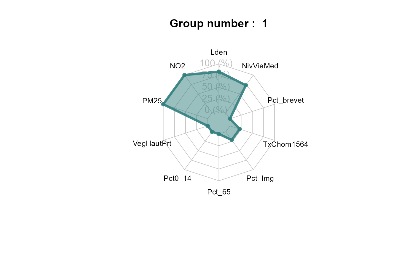

violinPlots(Data, SGFCM$Groups)

## [[1]]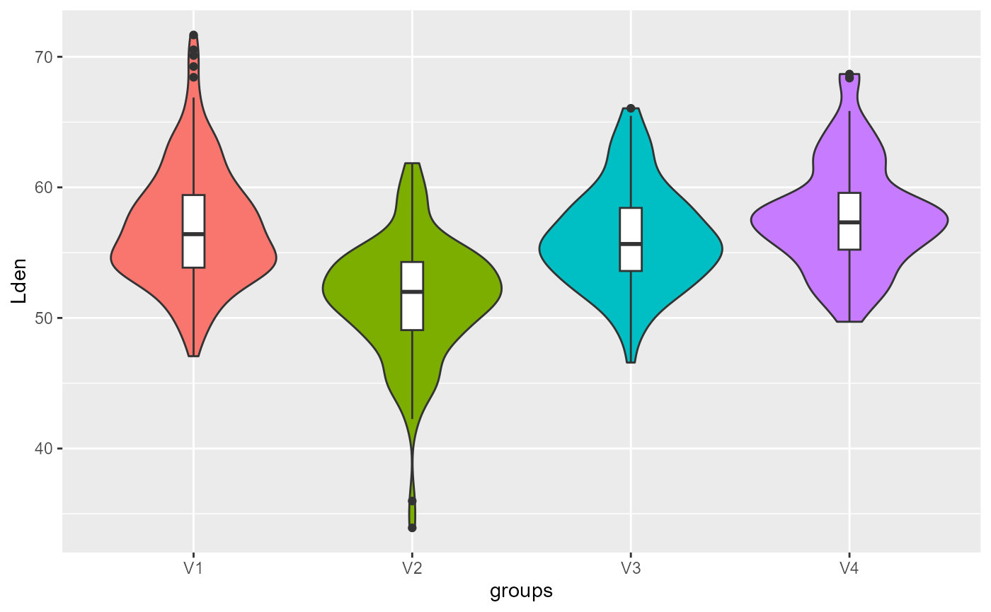

## 
## [[2]]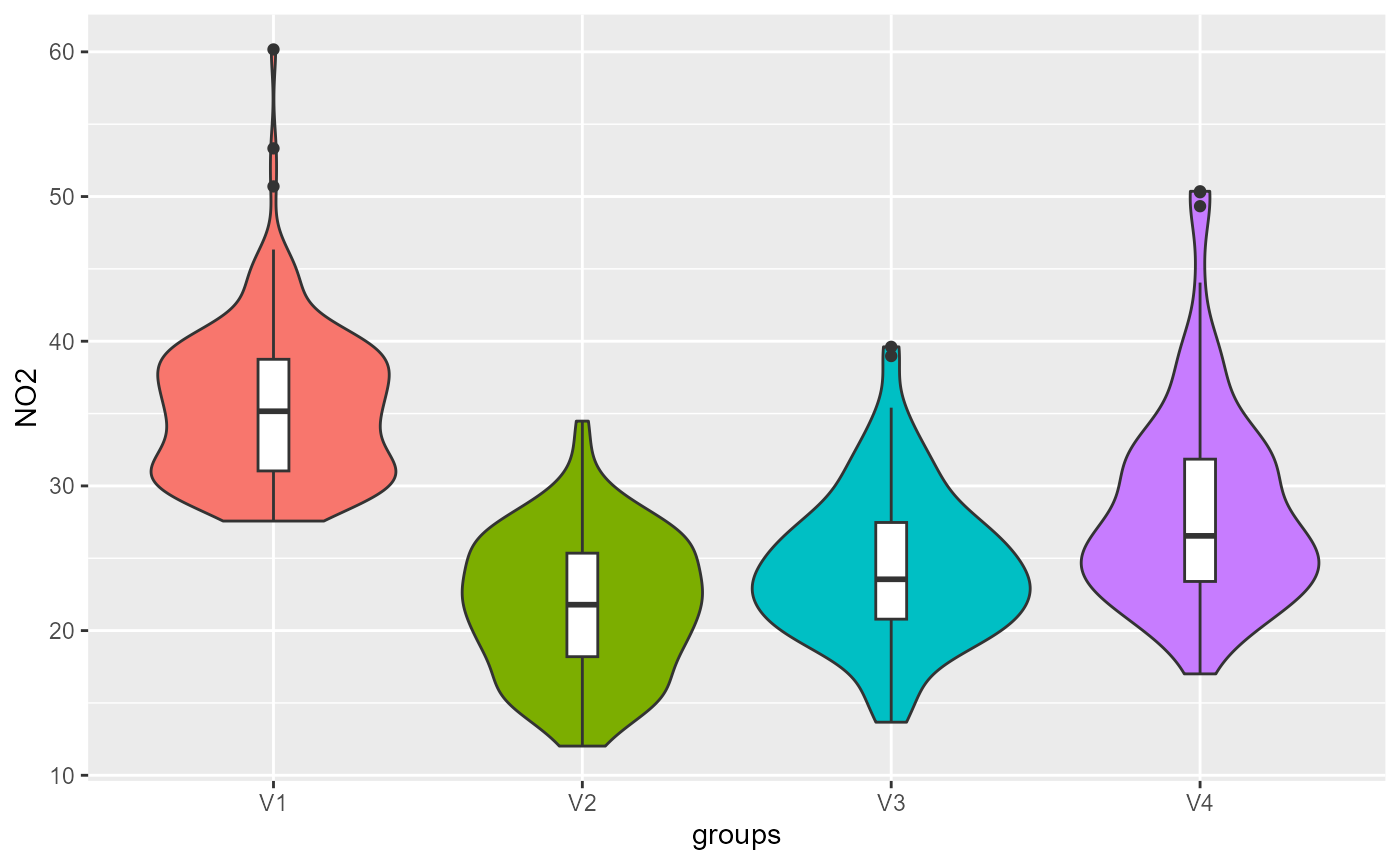

## 
## [[3]]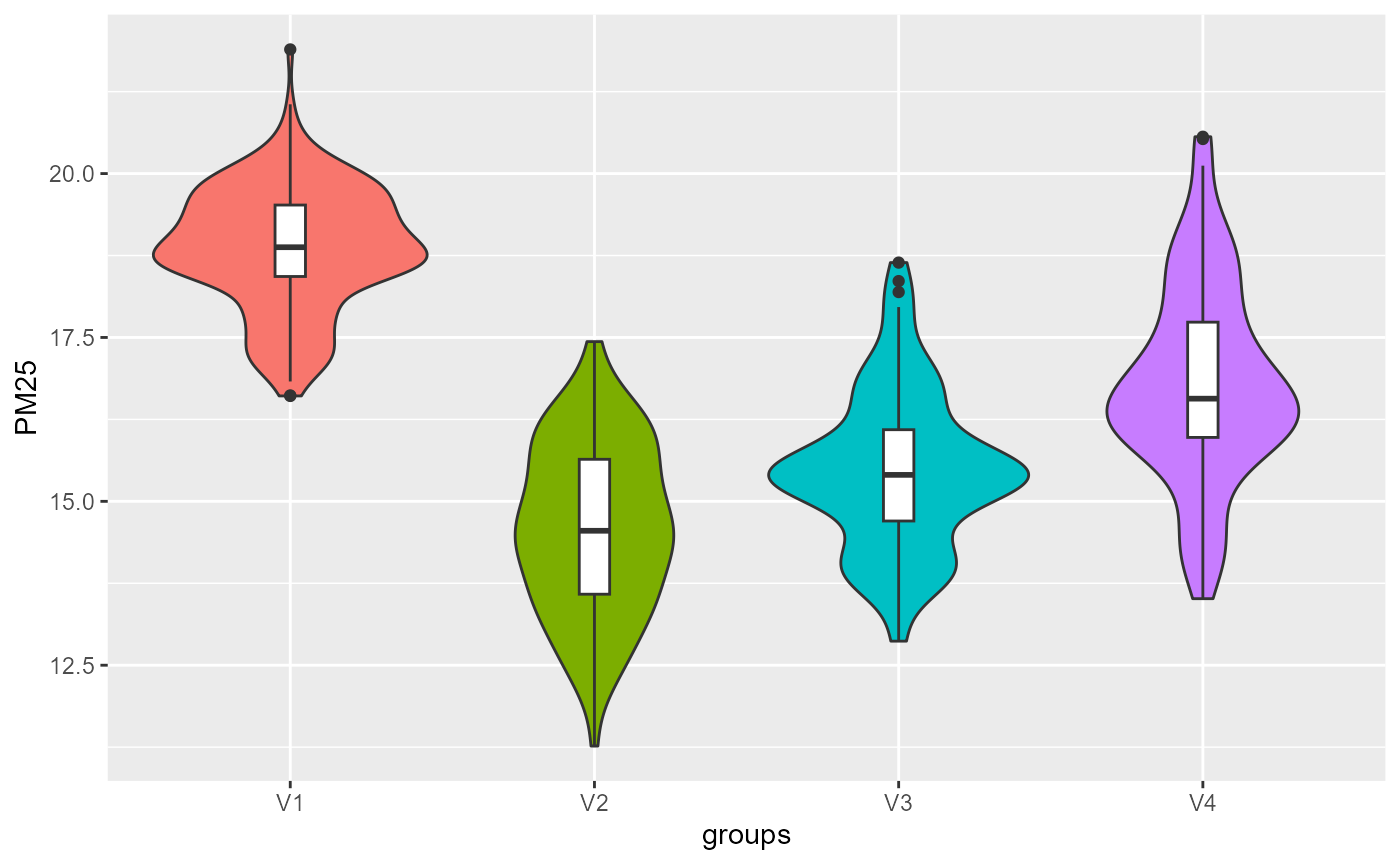

## 
## [[4]]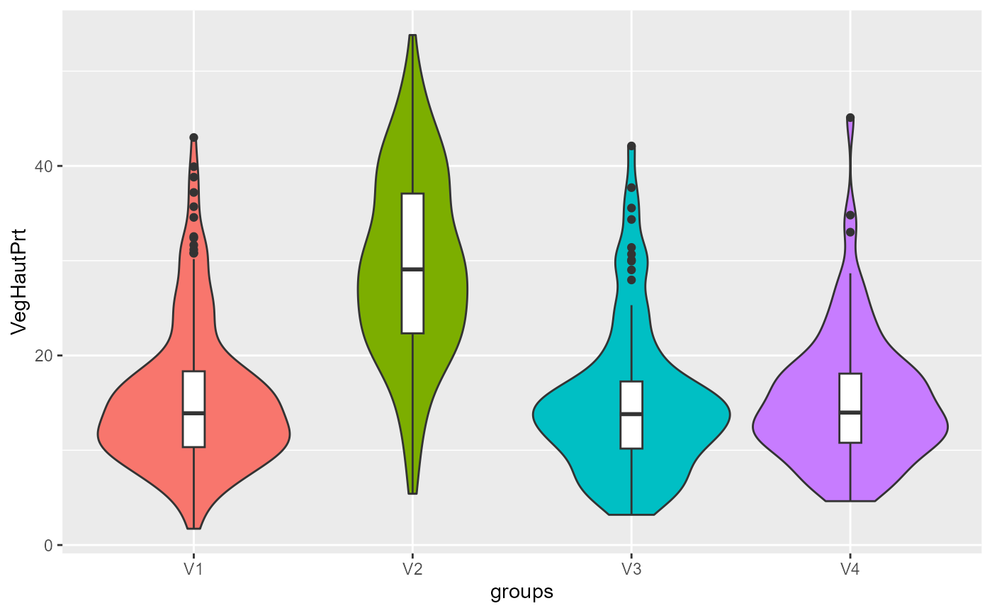

## 
## [[5]]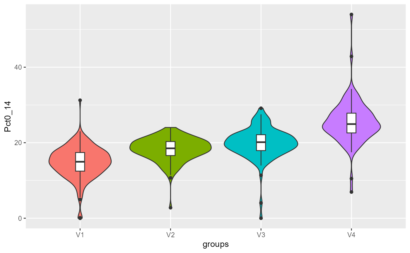

## 
## [[6]]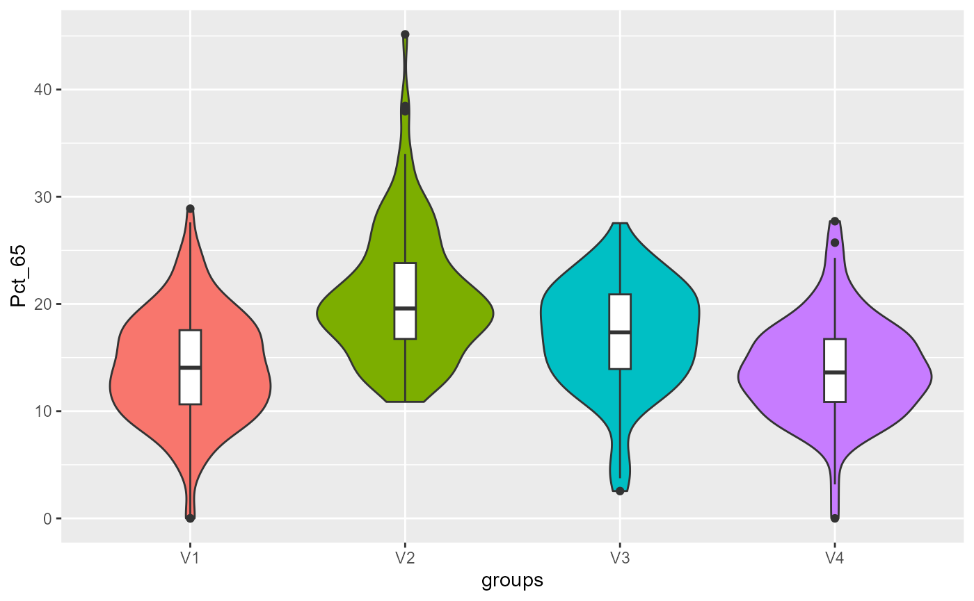

## 
## [[7]]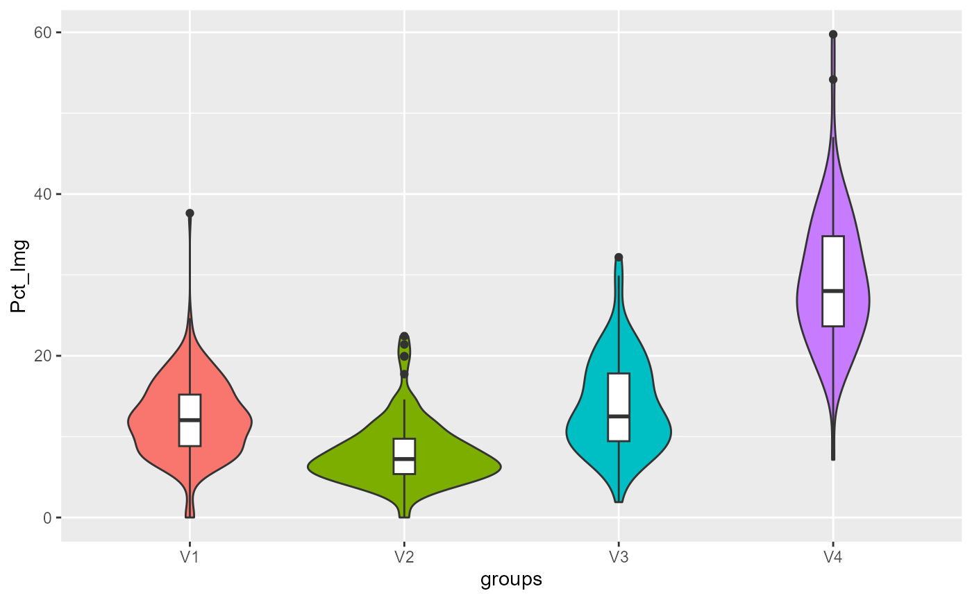

## 
## [[8]]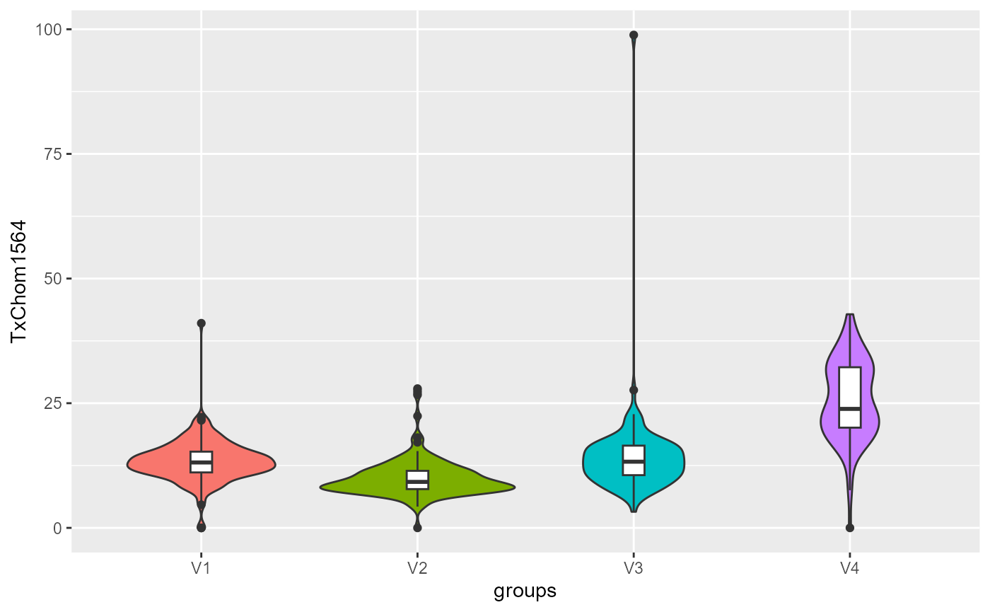

## 
## [[9]]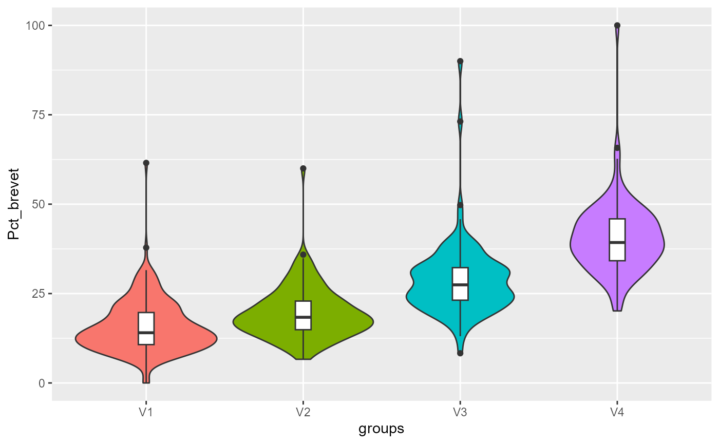

## 
## [[10]]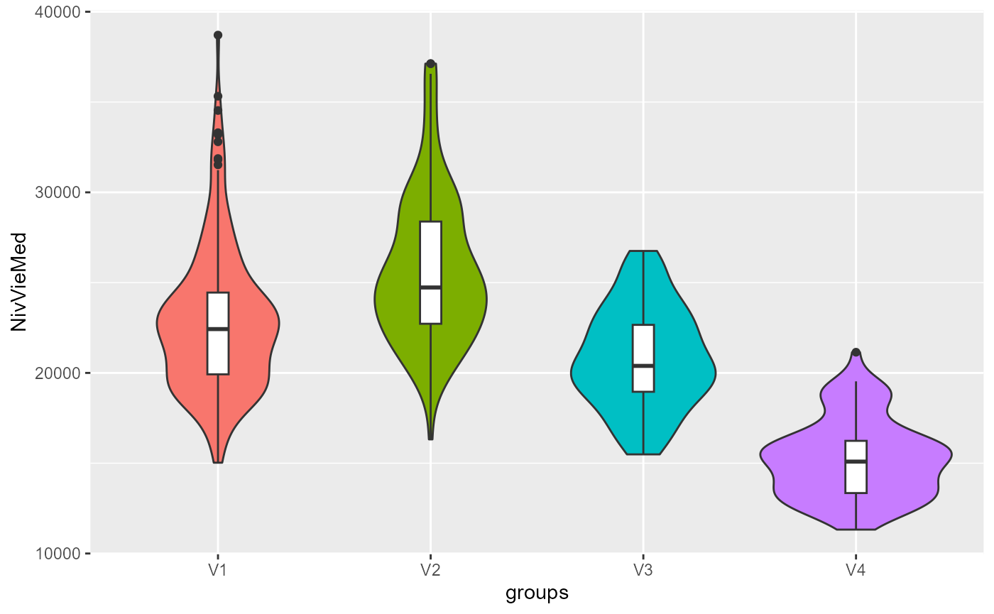

Ensuring clustering stability

All the clustering algorithms of this package depends on a initial state that might influence the results. A good practice is to check the results to ensure that the groups obtained are stable if we replicate the analysis. The function boost_group_validation proposes an approach based on bootstrapping.

bootvalues <- boot_group_validation(SGFCM, nsim = 1000, maxiter = 1000, 
                                     tol = 0.0001, verbose = FALSE)

We can now check if the groups are stable across simulations.

melted_df <- reshape2::melt(bootvalues$group_consistency)

## No id variables; using all as measure variables

melted_df$variable <- as.factor(melted_df$variable)

ggplot() +
  geom_histogram(mapping = aes(x = value), data = melted_df, bins = 30) +
  labs(title = "stability of clusters", subtitle = "for 1000 iterations",
       x = "Jaccard index") +
  facet_wrap(vars(variable), ncol=2)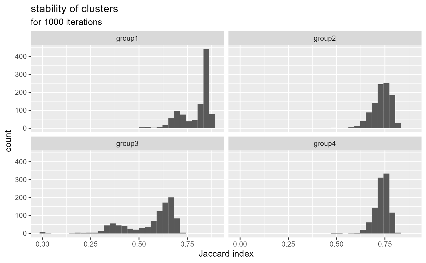

The Jaccard index is calculated at each replication and for each cluster in comparison with the original result. A greater value means a more stable cluster. Values above 0.75 indicate a stable cluster. Values between 0.5 and 0.75 indicate a cluster with some uncertainty. Under 0.5, the cluster tends to dissolve during the iterations. In the presented case, the group 3 is more worisome with many Jacard values under 0.5.

We can check the values of the centers of the group 3 across the 1000 iterations.

df_gp3 <- bootvalues$group_centers[["group3"]]

melted_df <- reshape2::melt(df_gp3)

## No id variables; using all as measure variables

melted_df$variable <- as.factor(melted_df$variable)

ggplot() +
  geom_histogram(mapping = aes(x = value), data = melted_df, bins = 30) +
  labs(title = "stability of group 3 centers", subtitle = "for 1000 iterations") +
  xlim(-3,3)+
  facet_wrap(vars(variable), ncol=3)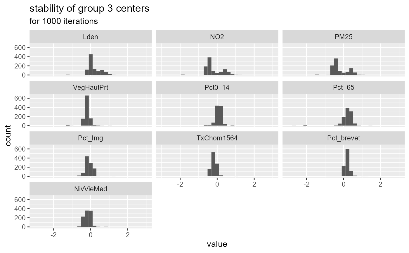

It appears that the center values for NO₂ and PM_2.5 are bimodal, that might explain why this group tends to dissolve. This could mean that group three is the combination of two very similar sub-groups.

Advanced example

SFCM with spatial non-local information

It has been proposed to modify the SFCM algorithm to include “non-local spatial information” instead of the information provided by close observations (Zhao, Liu, and Fan 2015). Basically, this implies a modified spatial weighting scheme combining neighbouring and semantic distance. This way, more similar neighbours get more weights in the calculation of the lagged dataset which can be desirable in dataset characterized by a lot of noise. When working with a classical vector dataset, one can use the function adjustSpatialWeights and create a row-standardized weight matrix using the inverse of the euclidean distance between observation and their neighbours as weights.

# create the modified weight matrix
WMat_adj <- adjustSpatialWeights(Data, WMat$neighbours, style = "W")

# calculate the modified version of FCM with non-local information
nl_SFCM <- SFCMeans(Data, WMat_adj, k = 4, m = 1.5, alpha = 0.7,
                 tol = 0.0001, standardize = FALSE,
                 verbose = FALSE, seed = 456)

When working with rasters, the same method can be apllied by giving "nl" as value for the parameter lag_method.

Reproductibility

Clustering methods like CMeans depend on the initial centers selected. In geocmeans, they are selected randomly, and two runs of the functions can yield different results. To facilitate the reproductibility of the results, the main functions of the package (CMeans, GFCMeans, SFCMeans, SGFCMeans, selectParameters, selectParameters.mc) have a seed parameter. It can be set by the user to ensure that the results of the functions are exactly the same.

Final words

That’s all, folks ! Following are the enhancements for the next version

introduce other methods of spatial c-means
open some other parameters to the user (such as the function defining the convergence criterion)
work on documentation

References

Cai, Weiling, Songcan Chen, and Daoqiang Zhang. 2007. “Fast and Robust Fuzzy c-Means Clustering Algorithms Incorporating Local Information for Image Segmentation.” Pattern Recognition 40 (3): 825–38.

Gelb, Jérémy, and Philippe Apparicio. 2021. “Apport de La Classification Floue c-Means Spatiale En géographie: Essai de Taxinomie Socio-résidentielle Et Environnementale à Lyon.” Cybergeo: European Journal of Geography.

Zhao, Feng, Licheng Jiao, and Hanqiang Liu. 2013. “Kernel Generalized Fuzzy c-Means Clustering with Spatial Information for Image Segmentation.” Digital Signal Processing 23 (1): 184–99.

Zhao, Feng, Hanqiang Liu, and Jiulun Fan. 2015. “A Multiobjective Spatial Fuzzy Clustering Algorithm for Image Segmentation.” Applied Soft Computing 30: 48–57.

Jeremy Gelb

02/04/2021