Spatio-temporal dbscan with network distance

Jeremy Gelb

2024-01-01

Introduction

This vignette is just a simple example about what can be done with spNetwork and little bit of imagination. We will performe here a spatio-temporal dbscan clustering with network distances on the bike_accident dataset. Here is the procedure:

1. calculating a network distance matrix between each pair of points;
2. calculating a temporal distance matrix between each pair of points;
3. Calculating a binary matrix as the intersection of the two previous matrices according to a temporal and a network maximum distance thresholds;
4. using the dbscan algorithm on the binary matrix;
5. analysing the results.

Calculating the two distance matrix

This is the first step, we will start with the network matrix.

# first load data and packages
library(sf)
library(spNetwork)
library(spdep)
library(dbscan)
library(tmap)

data(mtl_network)
data(bike_accidents)

distance_mat_listw <- network_listw(bike_accidents, mtl_network,
                                  maxdistance = 5000,
                                  dist_func = "identity",
                                  matrice_type = "I",
                                  grid_shape = c(1,1))

# spdep changed its name rom nb_list to neighbours
distance_mat_listw$neighbours <- distance_mat_listw$nb_list
distance_mat_net <- listw2mat(distance_mat_listw)

Great, now we will calculate a temporal distance matrix in days between the accidents.

bike_accidents$dt <- as.POSIXct(bike_accidents$Date, format = "%Y/%m/%d")
start_time <- min(bike_accidents$dt)
bike_accidents$time <- difftime(bike_accidents$dt,start_time, units = "day")

temporal_mat <- as.matrix(dist(bike_accidents$time))

Calculating the intersection matrix

We select here the two following thresholds: 500m and 25 days. We calculate a binary matrix indicating if two points are close enough in time and space to belong to the same cluster.

binary_mat <- as.integer(temporal_mat <= 25 & distance_mat_net<= 400)
dim(binary_mat) <- dim(temporal_mat)

Applying the dbscan algorithm

The last step is to just apply the dbscan algorithm!

result <- dbscan(binary_mat, eps = 1, minPts = 5)
result
#> DBSCAN clustering for 347 objects.
#> Parameters: eps = 1, minPts = 5
#> Using euclidean distances and borderpoints = TRUE
#> The clustering contains 4 cluster(s) and 325 noise points.
#> 
#>   0   1   2   3   4 
#> 325   7   5   5   5 
#> 
#> Available fields: cluster, eps, minPts, dist, borderPoints

Analysing the results

We will first map the clusters (everybody loves map).

tmap_mode("view")

bike_accidents$cluster <- as.character(result$cluster)
out_cluster <- subset(bike_accidents,bike_accidents$cluster == "0")
in_cluster <- subset(bike_accidents,bike_accidents$cluster != "0")

tm_shape(out_cluster) + 
  tm_dots("black", alpha = 0.3, size = 0.01) + 
  tm_shape(in_cluster) + 
  tm_dots("cluster")

And finally, we will plot the time period of each cluster.

ggplot(in_cluster) + 
  geom_point(aes(x = dt, y = cluster, color = cluster)) +
  scale_x_datetime(date_labels = "%Y/%m")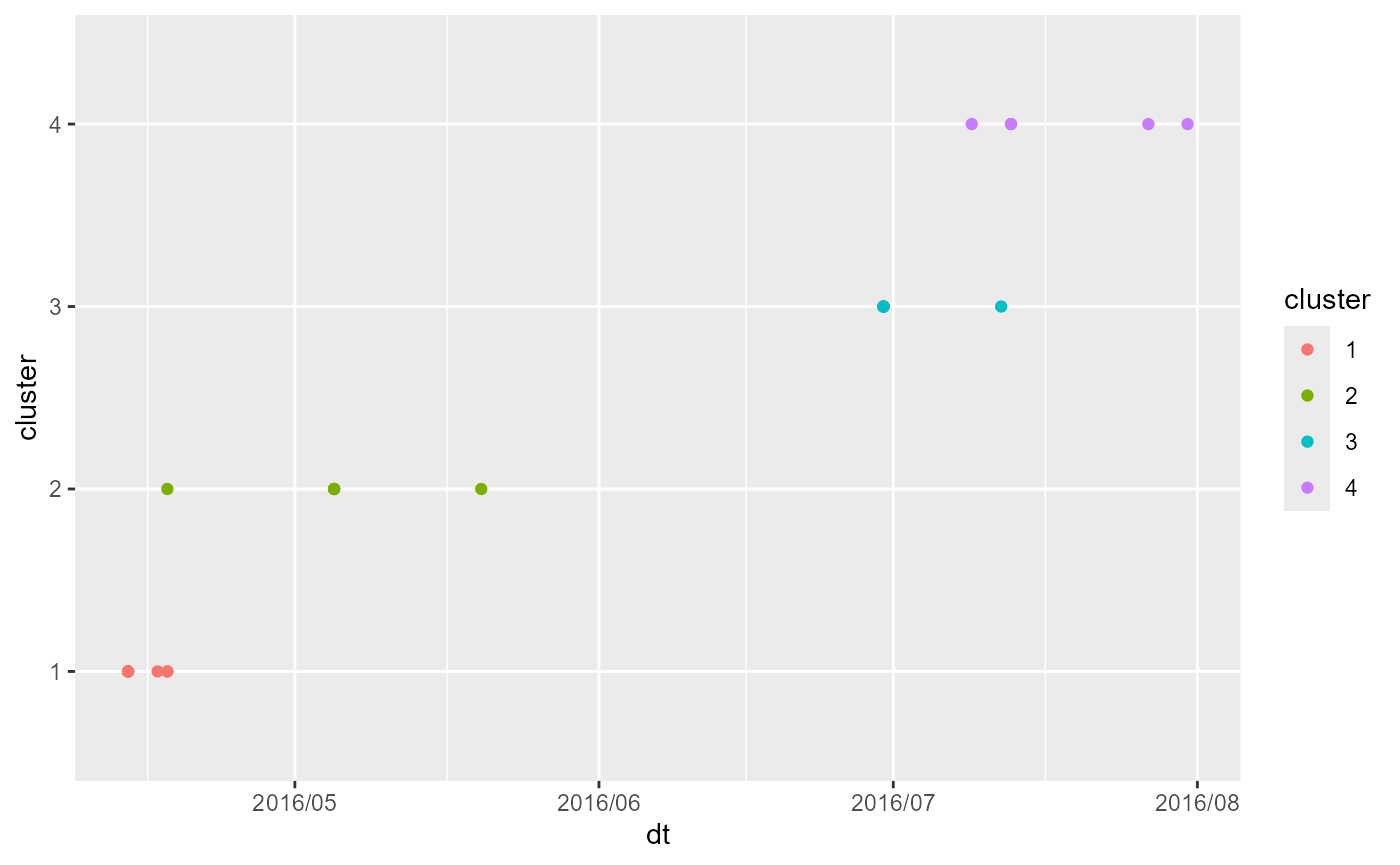

That’s all folks! I hope this short example was interesting!