Creating a FCMres object

Jeremy Gelb

02/04/2021

Introduction

In this vignette, we want to show how to create a FCMres object from results obtained with other classification or clustering methods. This can be very useful to compare results with methods available in other packages. We give a practical example here with the hclust function.

Applying hclust

We start by clustering the observations in the LyonIris dataset with the hclust function and retaining 4 groups.

library(geocmeans)
library(tmap)
library(dplyr)
library(ggplot2)
library(spdep)
library(terra)
library(sf)

data("LyonIris")

# selecting the columns for the analysis
AnalysisFields <- c("Lden","NO2","PM25","VegHautPrt","Pct0_14",
                   "Pct_65","Pct_Img","TxChom1564","Pct_brevet","NivVieMed")

# rescaling the columns
Data <- st_drop_geometry(LyonIris[AnalysisFields])
for (Col in names(Data)){
  Data[[Col]] <- scale(Data[[Col]])
}

# applying the hclust function
clust <- hclust(dist(Data), method = "ward")

# getting the groups
LyonIris$Hclust_groups <- as.character(cutree(clust, k = 4))
Data$Hclust_groups <- as.character(cutree(clust, k = 4))

# mapping the groups
tm_shape(LyonIris) + 
  tm_polygons(col = "Hclust_groups", title = "groups")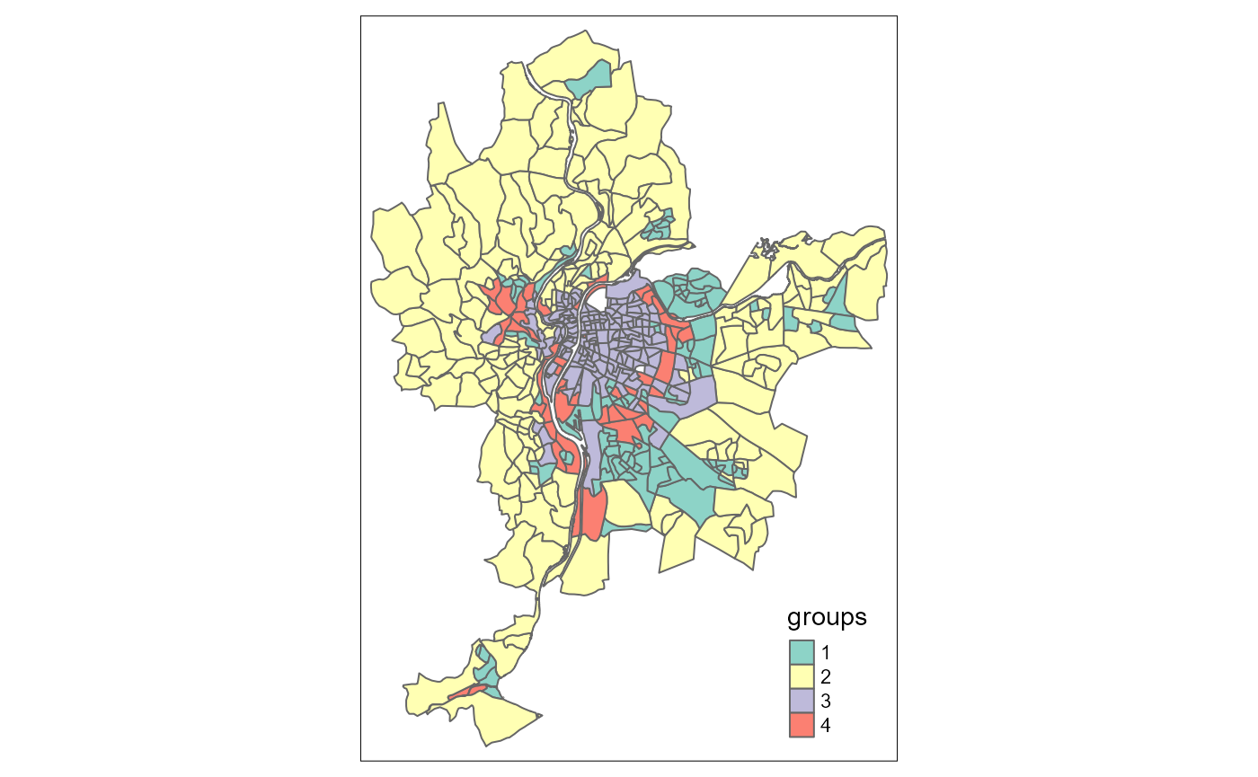

Creating a FCMres object

Now, if we want to use the functions provided by geocemans, we must create a FCMres object manually. This is basically a list with some required slots:

• Centers: a matrix representing the centre of each group
• Belongings: a membership matrix of each observation to each group
• Data: the dataset used for the clustering
• m: the fuzzyness factor (1 if using a hard clustering method)

In this case, we calculate the centres of the groups as the mean of each variable in each group.

centers <- Data %>% 
  group_by(Hclust_groups) %>%
  summarise_all(mean)

centers <- as.matrix(centers[2:ncol(centers)])

The membership matrix is a simple binary matrix. We can create it with the function cat_to_belongings.

member_mat <- cat_to_belongings(Data$Hclust_groups)

And we can now create our FCMres object.

Data$Hclust_groups <- NULL

hclustres <- FCMres(list(
  "Centers" = centers,
  "Belongings" = member_mat,
  "Data" = Data,
  "m" = 1,
  "algo" = "hclust"
))

It is now possible to use almost all the functions in the geocmeans package to investigate the results.

# quick summaries about the groups
summary(hclustres)
violinPlots(hclustres$Data, hclustres$Groups)
spiderPlots(hclustres$Data, hclustres$Belongings)
mapClusters(LyonIris, hclustres)

# some indices about classification quality
calcqualityIndexes(hclustres$Data,
                   hclustres$Belongings, 
                   hclustres$m)

# spatial diagnostic
Neighbours <- poly2nb(LyonIris,queen = TRUE)
WMat <- nb2listw(Neighbours,style="W",zero.policy = TRUE)
spatialDiag(hclustres, nblistw = WMat)

# investigation with the shiny app
sp_clust_explorer(hclustres, spatial = LyonIris)

Creating a FCMres object when working with rasters

When working with raster data, a little more work must be done to create a FCMres object. We show here a complete example with the Arcachon dataset.

We start here by applying the k-means algorithm to a set of rasters.

Arcachon <- terra::rast(system.file("extdata/Littoral4_2154.tif", package = "geocmeans"))
names(Arcachon) <- c("blue", "green", "red", "infrared", "SWIR1", "SWIR2")

# loading each raster as a column in a matrix
# and scale each column
all_data <- do.call(cbind, lapply(names(Arcachon), function(n){
  rast <- Arcachon[[n]]
  return(terra::values(terra::scale(rast), mat = FALSE))
}))

# removing the rows with missing values
missing <- complete.cases(all_data)
all_data <- all_data[missing,]

# applying the kmeans algorithm with 7 groups
kmean7 <- kmeans(all_data, 7)

We must now create three objects:

• Data: a list of rasterLayers with the values used in the clustering algorithm.
• rasters: a list of rasterLayers with the membership values of each pixel for each group.
• Centers: a matrix with the centres of each group.

# creating Data (do not forget the standardization)
Data <- lapply(names(Arcachon), function(n){
  rast <- Arcachon[[n]]
  return(terra::scale(rast))
})
names(Data) <- names(Arcachon)

# creating rasters
ref_raster <- Arcachon[[1]]

rasters <- lapply(1:7, function(i){
  # creating a vector with only 0 values
  vals <- rep(0, terra::ncell(ref_raster))
  # filling it with values when the pixels are not NA
  vals[missing] <- ifelse(kmean7$cluster == i,1,0)
  # setting the values in a rasterLayer
  rast <- ref_raster
  terra::values(rast) <- vals
  return(rast)
})

# creating centers
all_data <- as.data.frame(all_data)
names(all_data) <- names(Arcachon)
all_data$kmean_groups <- as.character(kmean7$cluster)

centers <- all_data %>% 
  group_by(kmean_groups) %>%
  summarise_all(mean)

centers <- as.matrix(centers[2:ncol(centers)])

We can now create a FCMres object !

myFCMres <- FCMres(list(
  "Data" = Data,
  "Centers" = centers,
  "rasters" = rasters,
  "m" = 1,
  "algo" = "kmeans"
))

And again, we can use the functions provided in geocmeans !

# quick summaries about the groups
summary(myFCMres)
violinPlots(myFCMres$Data, myFCMres$Groups)
spiderPlots(myFCMres$Data, myFCMres$Belongings)
mapClusters(object = myFCMres)

# some indices about classification quality
calcqualityIndexes(myFCMres$Data,
                   myFCMres$Belongings, 
                   myFCMres$m)

# spatial diagnostic
w1 <- matrix(1, nrow = 3, ncol = 3)
spatialDiag(myFCMres, window = w1, nrep = 5)

# investigation with the shiny app
sp_clust_explorer(myFCMres)